Multiscale analysis reveals that diet-dependent gut plasticity emerges from alterations in both stem cell niche coupling and enterocyte size.
Last updated: 2021-10-08
Checks: 6 1
Knit directory: Bonfini_eLife_2021/
This reproducible R Markdown analysis was created with workflowr (version 1.6.2). The Checks tab describes the reproducibility checks that were applied when the results were created. The Past versions tab lists the development history.
Great! Since the R Markdown file has been committed to the Git repository, you know the exact version of the code that produced these results.
Great job! The global environment was empty. Objects defined in the global environment can affect the analysis in your R Markdown file in unknown ways. For reproduciblity it’s best to always run the code in an empty environment.
The command set.seed(20211008) was run prior to running the code in the R Markdown file. Setting a seed ensures that any results that rely on randomness, e.g. subsampling or permutations, are reproducible.
Great job! Recording the operating system, R version, and package versions is critical for reproducibility.
Nice! There were no cached chunks for this analysis, so you can be confident that you successfully produced the results during this run.
Using absolute paths to the files within your workflowr project makes it difficult for you and others to run your code on a different machine. Change the absolute path(s) below to the suggested relative path(s) to make your code more reproducible.
| absolute | relative |
|---|---|
| F:/Dropbox/Github/Bonfini_eLife_2021/data/ | data |
| F:/Dropbox/Github/Bonfini_eLife_2021/data/1A.jpg | data/1A.jpg |
| F:/Dropbox/Github/Bonfini_eLife_2021/data/1C.jpg | data/1C.jpg |
| F:/Dropbox/Github/Bonfini_eLife_2021/data/1D.jpg | data/1D.jpg |
| F:/Dropbox/Github/Bonfini_eLife_2021/data/Figures/Figure_1.tiff | data/Figures/Figure_1.tiff |
| F:/Dropbox/Github/Bonfini_eLife_2021/data/Figures/Figure_1S1.tiff | data/Figures/Figure_1S1.tiff |
| F:/Dropbox/Github/Bonfini_eLife_2021/data/1- S2A.jpg | data/1- S2A.jpg |
| F:/Dropbox/Github/Bonfini_eLife_2021/data/Plot_Fig1S2B.jpeg | data/Plot_Fig1S2B.jpeg |
| F:/Dropbox/Github/Bonfini_eLife_2021/data/Figures/Figure_1S2.tiff | data/Figures/Figure_1S2.tiff |
| F:/Dropbox/Github/Bonfini_eLife_2021/data/1 - S3.jpg | data/1 - S3.jpg |
| F:/Dropbox/Github/Bonfini_eLife_2021/data/Figures/Figure_1S3.tiff | data/Figures/Figure_1S3.tiff |
| F:/Dropbox/Github/Bonfini_eLife_2021/data/Plot_Fig2A.jpeg | data/Plot_Fig2A.jpeg |
| F:/Dropbox/Github/Bonfini_eLife_2021/data/Nutri_geo_graph.jpg | data/Nutri_geo_graph.jpg |
| F:/Dropbox/Github/Bonfini_eLife_2021/data/Figures/Figure_2.tiff | data/Figures/Figure_2.tiff |
| F:/Dropbox/Github/Bonfini_eLife_2021/data/Plot_Fig2-S1B.jpeg | data/Plot_Fig2-S1B.jpeg |
| F:/Dropbox/Github/Bonfini_eLife_2021/data/Figures/Figure_2S1.tiff | data/Figures/Figure_2S1.tiff |
| F:/Dropbox/Github/Bonfini_eLife_2021/data/Figures/Figure_2S2.tiff | data/Figures/Figure_2S2.tiff |
| F:/Dropbox/Github/Bonfini_eLife_2021/data/3A.jpg | data/3A.jpg |
| F:/Dropbox/Github/Bonfini_eLife_2021/data/3B.jpg | data/3B.jpg |
| F:/Dropbox/Github/Bonfini_eLife_2021/data/3E.jpg | data/3E.jpg |
| F:/Dropbox/Github/Bonfini_eLife_2021/data/3F.jpg | data/3F.jpg |
| F:/Dropbox/Github/Bonfini_eLife_2021/data/Figures/Figure_3.tiff | data/Figures/Figure_3.tiff |
| F:/Dropbox/Github/Bonfini_eLife_2021/data/3 - S1B.jpg | data/3 - S1B.jpg |
| F:/Dropbox/Github/Bonfini_eLife_2021/data/3 - S1D.jpg | data/3 - S1D.jpg |
| F:/Dropbox/Github/Bonfini_eLife_2021/data/3 - S1E.jpg | data/3 - S1E.jpg |
| F:/Dropbox/Github/Bonfini_eLife_2021/data/3 - S1F.jpg | data/3 - S1F.jpg |
| F:/Dropbox/Github/Bonfini_eLife_2021/data/3 - S1G.jpg | data/3 - S1G.jpg |
| F:/Dropbox/Github/Bonfini_eLife_2021/data/Figures/Figure_3S1.tiff | data/Figures/Figure_3S1.tiff |
| F:/Dropbox/Github/Bonfini_eLife_2021/data/4E.jpg | data/4E.jpg |
| F:/Dropbox/Github/Bonfini_eLife_2021/data/4F.jpg | data/4F.jpg |
| F:/Dropbox/Github/Bonfini_eLife_2021/data/4G.jpg | data/4G.jpg |
| F:/Dropbox/Github/Bonfini_eLife_2021/data/4H.jpg | data/4H.jpg |
| F:/Dropbox/Github/Bonfini_eLife_2021/data/4I.jpg | data/4I.jpg |
| F:/Dropbox/Github/Bonfini_eLife_2021/data/4J.jpg | data/4J.jpg |
| F:/Dropbox/Github/Bonfini_eLife_2021/data/Figures/Figure_4.tiff | data/Figures/Figure_4.tiff |
| F:/Dropbox/Github/Bonfini_eLife_2021/data/4 - S1B.jpg | data/4 - S1B.jpg |
| F:/Dropbox/Github/Bonfini_eLife_2021/data/Plot_Fig4-S1F.jpeg | data/Plot_Fig4-S1F.jpeg |
| F:/Dropbox/Github/Bonfini_eLife_2021/data/Figures/Figure_4S1.tiff | data/Figures/Figure_4S1.tiff |
| F:/Dropbox/Github/Bonfini_eLife_2021/data/4 - S2A.jpg | data/4 - S2A.jpg |
| F:/Dropbox/Github/Bonfini_eLife_2021/data/Figures/Figure_4S2.tiff | data/Figures/Figure_4S2.tiff |
| F:/Dropbox/Github/Bonfini_eLife_2021/data/5C.jpg | data/5C.jpg |
| F:/Dropbox/Github/Bonfini_eLife_2021/data/5F.jpg | data/5F.jpg |
| F:/Dropbox/Github/Bonfini_eLife_2021/data/5F | data/5F |
| F:/Dropbox/Github/Bonfini_eLife_2021/data/5G.jpg | data/5G.jpg |
| F:/Dropbox/Github/Bonfini_eLife_2021/data/5G | data/5G |
| F:/Dropbox/Github/Bonfini_eLife_2021/data/5I.jpg | data/5I.jpg |
| F:/Dropbox/Github/Bonfini_eLife_2021/data/5I | data/5I |
| F:/Dropbox/Github/Bonfini_eLife_2021/data/5J.jpg | data/5J.jpg |
| F:/Dropbox/Github/Bonfini_eLife_2021/data/5J | data/5J |
| F:/Dropbox/Github/Bonfini_eLife_2021/data/Figures/Figure_5.tiff | data/Figures/Figure_5.tiff |
| F:/Dropbox/Github/Bonfini_eLife_2021/data/Figures/Figure_5S1.tiff | data/Figures/Figure_5S1.tiff |
| F:/Dropbox/Github/Bonfini_eLife_2021/data/5 - S2A.jpg | data/5 - S2A.jpg |
| F:/Dropbox/Github/Bonfini_eLife_2021/data/5 - S2A | data/5 - S2A |
| F:/Dropbox/Github/Bonfini_eLife_2021/data/5 - S2B.jpg | data/5 - S2B.jpg |
| F:/Dropbox/Github/Bonfini_eLife_2021/data/5 - S2B | data/5 - S2B |
| F:/Dropbox/Github/Bonfini_eLife_2021/data/5 - S2C.jpg | data/5 - S2C.jpg |
| F:/Dropbox/Github/Bonfini_eLife_2021/data/5 - S2C | data/5 - S2C |
| F:/Dropbox/Github/Bonfini_eLife_2021/data/5 - S2D.jpg | data/5 - S2D.jpg |
| F:/Dropbox/Github/Bonfini_eLife_2021/data/5 - S2D | data/5 - S2D |
| F:/Dropbox/Github/Bonfini_eLife_2021/data/Figures/Figure_5S2.tiff | data/Figures/Figure_5S2.tiff |
| F:/Dropbox/Github/Bonfini_eLife_2021/data/6B.jpg | data/6B.jpg |
| F:/Dropbox/Github/Bonfini_eLife_2021/data/6C.jpg | data/6C.jpg |
| F:/Dropbox/Github/Bonfini_eLife_2021/data/6H.jpg | data/6H.jpg |
| F:/Dropbox/Github/Bonfini_eLife_2021/data/6I.jpg | data/6I.jpg |
| F:/Dropbox/Github/Bonfini_eLife_2021/data/Figures/Figure_6.tiff | data/Figures/Figure_6.tiff |
| F:/Dropbox/Github/Bonfini_eLife_2021/data/6 - S1B.jpg | data/6 - S1B.jpg |
| F:/Dropbox/Github/Bonfini_eLife_2021/data/6 - S1C.jpg | data/6 - S1C.jpg |
| F:/Dropbox/Github/Bonfini_eLife_2021/data/6 - S1D.jpg | data/6 - S1D.jpg |
| F:/Dropbox/Github/Bonfini_eLife_2021/data/6 - S1E.jpg | data/6 - S1E.jpg |
| F:/Dropbox/Github/Bonfini_eLife_2021/data/Figures/Figure_6S1.tiff | data/Figures/Figure_6S1.tiff |
| F:/Dropbox/Github/Bonfini_eLife_2021/data/7B.jpg | data/7B.jpg |
| F:/Dropbox/Github/Bonfini_eLife_2021/data/7C.jpg | data/7C.jpg |
| F:/Dropbox/Github/Bonfini_eLife_2021/data/7E.jpg | data/7E.jpg |
| F:/Dropbox/Github/Bonfini_eLife_2021/data/7F.jpg | data/7F.jpg |
| F:/Dropbox/Github/Bonfini_eLife_2021/data/7I.jpg | data/7I.jpg |
| F:/Dropbox/Github/Bonfini_eLife_2021/data/Figures/Figure_7.tiff | data/Figures/Figure_7.tiff |
| F:/Dropbox/Github/Bonfini_eLife_2021/data/Figures/Figure_7S1.tiff | data/Figures/Figure_7S1.tiff |
| F:/Dropbox/Github/Bonfini_eLife_2021/data/7- S2A.jpg | data/7- S2A.jpg |
| F:/Dropbox/Github/Bonfini_eLife_2021/data/7- S2A1.jpg | data/7- S2A1.jpg |
| F:/Dropbox/Github/Bonfini_eLife_2021/data/7- S2B.jpg | data/7- S2B.jpg |
| F:/Dropbox/Github/Bonfini_eLife_2021/data/7- S2B1.jpg | data/7- S2B1.jpg |
| F:/Dropbox/Github/Bonfini_eLife_2021/data/Figures/Figure_7S2.tiff | data/Figures/Figure_7S2.tiff |
| F:/Dropbox/Github/Bonfini_eLife_2021/data/7 - S3A.jpg | data/7 - S3A.jpg |
| F:/Dropbox/Github/Bonfini_eLife_2021/data/Figures/Figure_7S3.tiff | data/Figures/Figure_7S3.tiff |
Great! You are using Git for version control. Tracking code development and connecting the code version to the results is critical for reproducibility.
The results in this page were generated with repository version 2e08f0d. See the Past versions tab to see a history of the changes made to the R Markdown and HTML files.
Note that you need to be careful to ensure that all relevant files for the analysis have been committed to Git prior to generating the results (you can use wflow_publish or wflow_git_commit). workflowr only checks the R Markdown file, but you know if there are other scripts or data files that it depends on. Below is the status of the Git repository when the results were generated:
Ignored files:
    Ignored:    data/.Rhistory

Untracked files:
    Untracked:  data/.RDataTmp
    Untracked:  data/.RDataTmp1
    Untracked:  data/.RDataTmp2
    Untracked:  data/.RDataTmp3
    Untracked:  data/.RDataTmp4
    Untracked:  data/.RDataTmp5
    Untracked:  data/.RDataTmp6
    Untracked:  data/.RDataTmp7
    Untracked:  data/1 - S1B.csv
    Untracked:  data/1 - S1C.csv
    Untracked:  data/1 - S1D.csv
    Untracked:  data/1 - S1E.csv
    Untracked:  data/1 - S3.jpg
    Untracked:  data/1- S2A.jpg
    Untracked:  data/1A.jpg
    Untracked:  data/1B.csv
    Untracked:  data/1C.jpg
    Untracked:  data/1D.jpg
    Untracked:  data/1E - 1S1A.csv
    Untracked:  data/1F - G.csv
    Untracked:  data/2 - S1A.csv
    Untracked:  data/2 - S2A.csv
    Untracked:  data/2 - S2B.csv
    Untracked:  data/2 -S1B supplement data.xlsx
    Untracked:  data/2-S1C.csv
    Untracked:  data/2A.csv
    Untracked:  data/2E - calories.csv
    Untracked:  data/2E - table.tif
    Untracked:  data/2E.csv
    Untracked:  data/2F - calories.csv
    Untracked:  data/2F.csv
    Untracked:  data/2G.csv
    Untracked:  data/2S2C.csv
    Untracked:  data/3 - S1A.csv
    Untracked:  data/3 - S1B.jpg
    Untracked:  data/3 - S1C.csv
    Untracked:  data/3 - S1D.jpg
    Untracked:  data/3 - S1E.jpg
    Untracked:  data/3 - S1F.jpg
    Untracked:  data/3 - S1G.jpg
    Untracked:  data/3 - S1H.csv
    Untracked:  data/3A.jpg
    Untracked:  data/3B.jpg
    Untracked:  data/3C.csv
    Untracked:  data/3E.jpg
    Untracked:  data/3F.jpg
    Untracked:  data/3G.csv
    Untracked:  data/3H.csv
    Untracked:  data/4 - S1A.csv
    Untracked:  data/4 - S1B.jpg
    Untracked:  data/4 - S1F.csv
    Untracked:  data/4 - S2A.jpg
    Untracked:  data/4A.csv
    Untracked:  data/4B, 4S1C.csv
    Untracked:  data/4C', 4S1D'.csv
    Untracked:  data/4C, 4S1D.csv
    Untracked:  data/4E.jpg
    Untracked:  data/4F.jpg
    Untracked:  data/4G.jpg
    Untracked:  data/4H.jpg
    Untracked:  data/4I.jpg
    Untracked:  data/4J.jpg
    Untracked:  data/4K.csv
    Untracked:  data/4L, 4S2D.csv
    Untracked:  data/4S2B.csv
    Untracked:  data/4S2C.csv
    Untracked:  data/5 - S1A.csv
    Untracked:  data/5 - S2A'.jpg
    Untracked:  data/5 - S2A.jpg
    Untracked:  data/5 - S2B'.jpg
    Untracked:  data/5 - S2B.jpg
    Untracked:  data/5 - S2C'.jpg
    Untracked:  data/5 - S2C.jpg
    Untracked:  data/5 - S2D'.jpg
    Untracked:  data/5 - S2D.jpg
    Untracked:  data/5 - S2E.csv
    Untracked:  data/5 - S2F.csv
    Untracked:  data/5 - S2G.csv
    Untracked:  data/5-S2.jpg
    Untracked:  data/5B.csv
    Untracked:  data/5C.jpg
    Untracked:  data/5C.xlsx
    Untracked:  data/5D.csv
    Untracked:  data/5E.csv
    Untracked:  data/5F'.jpg
    Untracked:  data/5F.jpg
    Untracked:  data/5G'.jpg
    Untracked:  data/5G.jpg
    Untracked:  data/5H.csv
    Untracked:  data/5I'.jpg
    Untracked:  data/5I.jpg
    Untracked:  data/5J'.jpg
    Untracked:  data/5J.jpg
    Untracked:  data/5K.csv
    Untracked:  data/5L.csv
    Untracked:  data/5M.csv
    Untracked:  data/6 - S1B.jpg
    Untracked:  data/6 - S1C.jpg
    Untracked:  data/6 - S1D.jpg
    Untracked:  data/6 - S1E.jpg
    Untracked:  data/6 - S1F.csv
    Untracked:  data/6A - 7A.csv
    Untracked:  data/6B.jpg
    Untracked:  data/6C.jpg
    Untracked:  data/6D.csv
    Untracked:  data/6E.csv
    Untracked:  data/6F.csv
    Untracked:  data/6G.csv
    Untracked:  data/6H.jpg
    Untracked:  data/6I.jpg
    Untracked:  data/6J.csv
    Untracked:  data/7 - S1A.csv
    Untracked:  data/7 - S2C.csv
    Untracked:  data/7 - S2D.csv
    Untracked:  data/7 - S2E.csv
    Untracked:  data/7 - S3A.jpg
    Untracked:  data/7- S2A.jpg
    Untracked:  data/7- S2A1.jpg
    Untracked:  data/7- S2B.jpg
    Untracked:  data/7- S2B1.jpg
    Untracked:  data/7B.jpg
    Untracked:  data/7C.jpg
    Untracked:  data/7D.csv
    Untracked:  data/7E.jpg
    Untracked:  data/7F.jpg
    Untracked:  data/7G.csv
    Untracked:  data/7H.csv
    Untracked:  data/7I.jpg
    Untracked:  data/7J.csv
    Untracked:  data/7K.csv
    Untracked:  data/7L.csv
    Untracked:  data/DGRP_wolbachia_DFD.csv
    Untracked:  data/GWAS_Response_Gut_Diet.jpg
    Untracked:  data/Plot_Fig1S2B.jpeg
    Untracked:  data/Plot_Fig2-S1B.jpeg
    Untracked:  data/Plot_Fig2A.jpeg
    Untracked:  data/Plot_Fig4-S1F.jpeg
    Untracked:  data/Template TIF.tif
    Untracked:  data/genes_info.csv
    Untracked:  data/gutGrowthDataIndex.csv
    Untracked:  data/image_5C.jpg
    Untracked:  data/normCounts.csv
    Untracked:  data/normCountsMeans_noDay4.csv
    Untracked:  data/readTable.csv
    Untracked:  data/readTableTMP.csv
    Untracked:  data/readTableTPM.csv
    Untracked:  data/stockDecode.csv
    Untracked:  data/weights.csv
Note that any generated files, e.g. HTML, png, CSS, etc., are not included in this status report because it is ok for generated content to have uncommitted changes.
These are the previous versions of the repository in which changes were made to the R Markdown (analysis/Bonfini_eLife_2021.Rmd) and HTML (docs/Bonfini_eLife_2021.html) files. If you’ve configured a remote Git repository (see ?wflow_git_remote), click on the hyperlinks in the table below to view the files as they were in that past version.
| File | Version | Author | Date | Message |
|---|---|---|---|---|
| Rmd | 2e08f0d | dduneau | 2021-10-08 | Bonfini eLife 2021 project |
| Rmd | e96cf31 | dduneau | 2021-10-08 | Update Bonfini_eLife_2021.Rmd |
| html | ec22c19 | dduneau | 2021-10-08 | Build site. |
| Rmd | 8fa9317 | dduneau | 2021-10-08 | Bonfini eLife 2021 project |
Table of contents
Library, Data import and reformatting
Library
library(devtools)
library(reshape2)
library(lattice)
library(MASS)
library(car)
library(lmtest)
library(ggplot2)
library(survival)
library(plotrix)
library(grid)
library(gridExtra)
library(agricolae)
library(nparLD)
library(psych)
library(doBy)
library(xlsxjars)
library(xlsx)
library(dplyr)
library(stringr)
library(scales)
library(tidyr)
library(phia)
library(data.table)
library(spaMM)
library(lme4)
library(fields)
library(EBImage)
library(gplots)
library(RColorBrewer)
library(gridGraphics)
library(fields)
library(multcomp)
library(ggrepel)
library(metR)
library(forcats)
library(ggh4x)#remotes::install_github("teunbrand/ggh4x")
library(GenomicRanges)
library(DESeq2)
library(RColorBrewer)
library(coxme)
library(ggplotify)
#library(base2grob)
library(knitr)
library(kableExtra)
library(plotfunctions)
library(ggsignif)
#Function to include factor that are NOT in a list
'%!in%' = function(x,y)!('%in%'(x,y))

#Function to Grab graph and display it as a ggplot graph
grab_grob = function(){
  grid.echo()
  grid.grab()
}


#Function to calculate standard deviaion
sd = function(x) sqrt(var(x,na.rm=T))


#Function to calculate standard error
se = function(x) sqrt(var(x,na.rm=T)/length(x))

# Function to graph survival with ggplot and displaying the checkpoints
ggplotprep2 <- function(x, times){
  #spreading the surfit dataframe into dataframe per day.
  d <- data.frame(condition=rep(names(x$strata), x$strata), time=x$time, survival=x$surv, upper=x$upper, lower=x$lower)
  # function to add time point 0
  fillup0 <- function(s) rbind(c(condition=s, time=0, survival=1, upper=1, lower=1), d[d$condition==s, ], deparse.level = 0)

  # function to determine the missing time points
  indexes <- function(x, time) {
    if(x%in%time) return(x)
    return(time[which.min(abs(time[time<x]-x))])
  }
  #Function to complete the missing time points
  fillup <- function(s) {
    d.temp <- d[d$condition==s, ]
    time <- as.numeric(d.temp$time)
    id <- sapply(times, indexes, time=time)
    d.temp <- d.temp[match(id, time), ]
    d.temp$time <- times
    return(d.temp)
  }

  if(times[1]==0) d <- do.call("rbind", sapply(names(x$strata), fillup0, simplify=F))
  d <- do.call("rbind", sapply(names(x$strata), fillup, simplify=F))
  clean.name <- function(name) unlist(lapply(strsplit(as.character(name), split="="), function(x) x[2]))
  d <- data.frame(Condition=clean.name(d$condition), Time=as.numeric(d$time), Survival=as.numeric(d$survival), upper=as.numeric(d$upper), lower=as.numeric(d$lower))
  return(d)
}


#function to select colours for GF-style plot (function mapping colors)
seeMahPal <- function(x, pal){
    pal[round(x)]
}

    #a function to take x,y,z
    #and return a GF-style plot with points per diet
geomPlotta <- function(x,y,z,alf,...){
    dat <- data.frame(x=x, y=y, z=z)
    d.means <- aggregate(z ~ x * y, dat, mean)
    surf.te <- Tps(cbind(dat$x, dat$y), dat$z, lambda = 0)

    experiColours <- data.frame(z=d.means$z, rank=rank(d.means$z), rnd=round(d.means$z), rankRnd=rank(round(d.means$z)))
    mahPal <- colorRampPalette(c("darkblue", "blue", "turquoise", "yellow", "orange", "red", "darkred"))(max(experiColours$rank)) #Decide colors

d.means$colour <- seeMahPal(x=d.means$z, pal=mahPal)

surface(predictSurface(surf.te, extrap=F), col=alpha(mahPal, alf), ...)
points(d.means$x, d.means$y, bg=seeMahPal(x=experiColours$rank, pal=mahPal), col="white", pch=21, cex=1, ...)
}


left = function(text, num_char) {
  substr(text, 1, num_char)
}

mid = function(text, start_num, num_char) {
  substr(text, start_num, start_num + num_char - 1)
}

right = function(text, num_char) {
  substr(text, nchar(text) - (num_char-1), nchar(text))
}
Font size and palettes
SuperSmallfont= 6
xSmallfont = 8
Smallfont= 10
Mediumfont= 12
Largefont= 14
verylargefont = 16
pointsize= 0.7
linesize=0.35
meansize = 1.5
Margin=c(0,0,0,0)

fontsizeaxes = 14
fontsizeaxes2 = 10

palette_diet_2 = c("#FFB4B4", "#C3E6FC")
palette_component_3 = c("#f4ead0","#2d5ad7","gold")
palette_mean = c("yellow","green","red","white","magenta","skyblue", "blue", "deeppink", "gold")
cbbPalette_4 = c("#BDE6BD", "#C3E6FC", "#FFE5E5", "#E5E5FF") #Green eclosion, HY, HYtoHS, HStoHY
cbbHS_HStoHY = c("#FFB4B4","#E5E5FF")
cbbHY_HYtoHS = c("#C3E6FC","#FFE5E5")
Warning: The above code chunk cached its results, but it won’t be re-run if previous chunks it depends on are updated. If you need to use caching, it is highly recommended to also set knitr::opts_chunk$set(autodep = TRUE) at the top of the file (in a chunk that is not cached). Alternatively, you can customize the option dependson for each individual chunk that is cached. Using either autodep or dependson will remove this warning. See the knitr cache options for more details.
Import dataset
path.to.data = "F:/Dropbox/Github/Bonfini_eLife_2021/data/"


rm(d,path)
d = list()
path = list()
for(f in list.files(path=path.to.data,pattern="*.csv$",recursive=T,full.names=T)) {
  nom = gsub(".*/(.*).csv","\\1",f)
  cat(nom,"\n")
  path[[nom]] = gsub("(.*)/.*csv","\\1/",f)
  d[[nom]] = read.table(f,header=T,sep=",")
}
Warning: The above code chunk cached its results, but it won’t be re-run if previous chunks it depends on are updated. If you need to use caching, it is highly recommended to also set knitr::opts_chunk$set(autodep = TRUE) at the top of the file (in a chunk that is not cached). Alternatively, you can customize the option dependson for each individual chunk that is cached. Using either autodep or dependson will remove this warning. See the knitr cache options for more details.
Data meaning - DGRP GWAS
wolb = d[["DGRP_wolbachia_DFD"]]
colnames(wolb) = c("dgrp_id", "wolbachia")
wolb$dgrp_id = gsub("line_", "DGRP-", wolb$dgrp_id)

weight = d[["weights"]]
decode = d[["stockDecode"]]

weight$mg = weight$weightPerFlyGram * 1000
weight$diet = tolower(weight$diet)
decode$shortID = as.factor(as.character(decode$shortID))
weight$stockNumber = as.factor(as.character(weight$dgrp))
weight = merge(weight, decode, by.x="stockNumber", by.y="shortID")
colnames(weight) = tolower(colnames(weight))
weight = weight[,which(!colnames(weight) %in% c("stockNumber", "dgrp.x"))]
colnames(weight)[which(colnames(weight) == "dgrp.y")] = "dgrp"
weight$dgrp_number = substr(as.character(weight$dgrp), 1, 3)
weight$dgrpDiet = factor(paste(weight$dgrp_number, weight$diet, sep="_"))

tab_GWAS_gut = d[["1F - G"]]

#edit the data
table(complete.cases(tab_GWAS_gut))
#str(tab_GWAS_gut)
tab_GWAS_gut= mutate_if(tab_GWAS_gut,is.integer,as.factor)

colnames(tab_GWAS_gut) = tolower(colnames(tab_GWAS_gut))
tab_GWAS_gut = tab_GWAS_gut[,!colnames(tab_GWAS_gut) %in% c("notes", "image", "bloomington_id")]

#remove the samples that subsequently proved crazy
tab_GWAS_gut = subset(tab_GWAS_gut, anteriorwidth < 1000)
tab_GWAS_gut = subset(tab_GWAS_gut, middlelength < 1500)

#remove lines that don't appear in both diets
dgrpLines = levels(tab_GWAS_gut$dgrp_number)
yDat = droplevels(subset(tab_GWAS_gut, diet=="y"))
xDat = droplevels(subset(tab_GWAS_gut, diet=="x"))
length(dgrpLines)
dgrpLines = dgrpLines[dgrpLines %in% yDat$dgrp_number]
#length(dgrpLines)
dgrpLines = dgrpLines[dgrpLines %in% xDat$dgrp_number]
#length(dgrpLines)

tab_GWAS_gut = droplevels(subset(tab_GWAS_gut, dgrp_number %in% dgrpLines))
yDat = droplevels(subset(yDat, dgrp_number %in% dgrpLines))
xDat = droplevels(subset(xDat, dgrp_number %in% dgrpLines))

#link up Wolbachia
tab_GWAS_gut = merge(tab_GWAS_gut, wolb, by="dgrp_id")
tab_GWAS_gut= mutate_if(tab_GWAS_gut,is.character,as.factor)
Warning: The above code chunk cached its results, but it won’t be re-run if previous chunks it depends on are updated. If you need to use caching, it is highly recommended to also set knitr::opts_chunk$set(autodep = TRUE) at the top of the file (in a chunk that is not cached). Alternatively, you can customize the option dependson for each individual chunk that is cached. Using either autodep or dependson will remove this warning. See the knitr cache options for more details.
1 Figure 1. Diet composition affects size and regional allometry of the midgut
1.1 Figure 1 - main
1.1.1 Figure 1A
Illustration of general dietary treatment design. Flies were reared on pre-experiment diet during development. At eclosion, flies were allocated to either HS or HY before midgut dissection at 5 days post eclosion.
img1A = readImage("F:/Dropbox/Github/Bonfini_eLife_2021/data/1A.jpg")
gob_imageFig1A = rasterGrob(img1A)
grid.draw(gob_imageFig1A)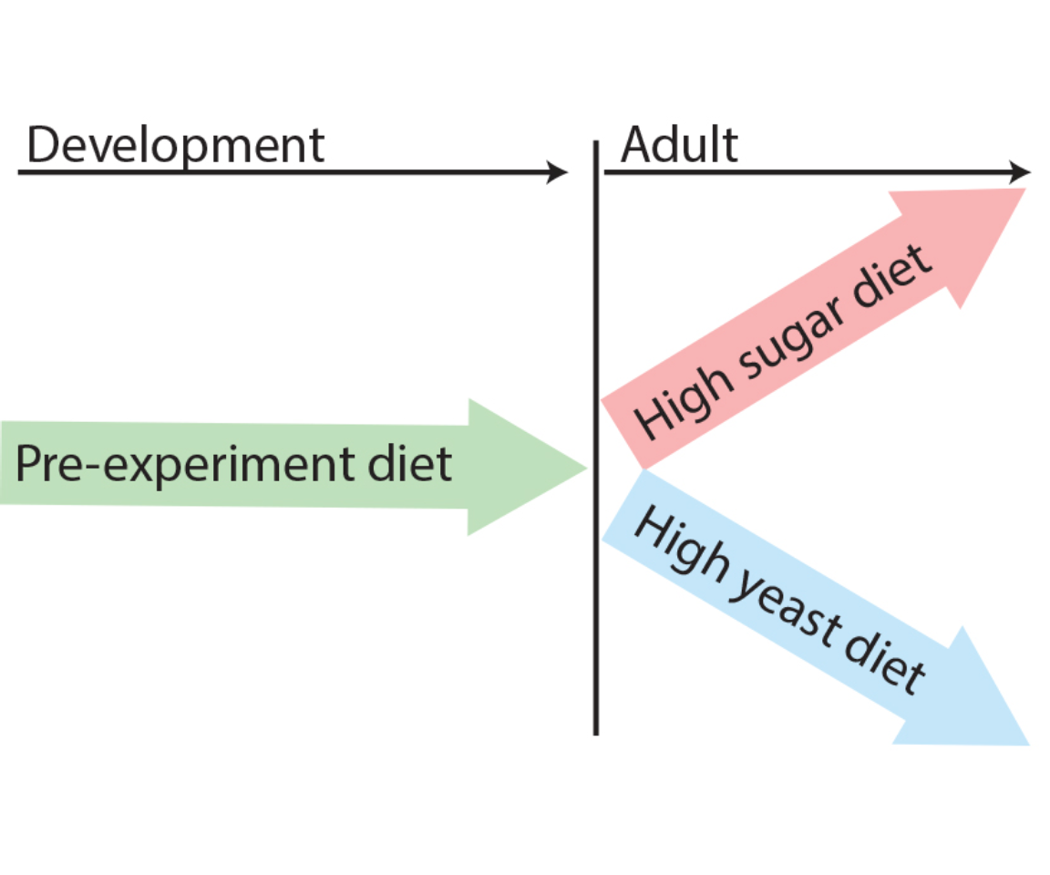
1.1.2 Figure 1B
Nutritional composition (proteins, carbohydrates, and lipids) of the two isocaloric diets used as a basis for this study as calories per liter of food: enriched in sugars (High sugar, HS) or yeast (High yeast, HY).
general_info_diet =d[["1B"]]
general_info_diet = mutate_if(general_info_diet,is.character,as.factor)

general_info_diet$Component <- factor(general_info_diet$Component, levels = c("Lipids","Proteins","Carbohydrates"))
Limits = c("Lipids","Proteins","Carbohydrates")
Labels = c("Lipids","Proteins","Carbohydrates")

Plot_Fig1B=
ggplot(general_info_diet,aes(x=Diet,y=Calories.contributed))+
geom_bar(stat="identity",aes(fill=Component),color="black",width=.90)+
  scale_fill_manual(limits=Limits,
                      values=palette_component_3,
                      labels=Labels)+
  scale_x_discrete("",
                     limits=c("HS", "HY"),
                     breaks=c("HS", "HY"))+
  scale_y_continuous("Calories/L of food",
                     breaks=c(seq(0,650,by=200),696))+
  theme(axis.title.x = element_text(size=Smallfont,colour="black"),
        axis.title.y =  element_text(size=Smallfont,colour="black"),
        axis.line.x = element_line(colour="black"),
        axis.line.y = element_line(colour="black"),
        axis.ticks.x = element_line(),
        axis.ticks.y = element_line(),
        axis.text.x = element_text(size=Smallfont,colour="black"),
        axis.text.y = element_text(size=Smallfont,colour="black"),
        panel.grid = element_blank(),
        plot.margin = unit(c(0,0,0,0), "cm"),
        legend.direction = "vertical",
        legend.box = "vertical",
        legend.position = c(0.5,-0.3),
        legend.key.height = unit(0.3, "cm"),
        legend.key.width= unit(0.3, "cm"),
        legend.margin=margin(t=-0.9, r=-0, b=-0, l=-0, unit="cm"),
        legend.title = element_blank(),
        legend.key = element_rect(colour = 'white', fill = "white", linetype='dashed'),
        legend.text = element_text(size=xSmallfont),
        legend.background = element_rect(fill=NA),
        strip.text.x = element_text(size =Smallfont, colour = "black",face="italic"),
        strip.text.y = element_text(size =Smallfont, colour = "black",face="italic"),
        strip.background = element_rect(fill=NA, colour="black"),
        strip.placement="outside",
        panel.background = element_rect(fill="transparent"))+
  guides(fill=guide_legend(ncol=1))
Plot_Fig1B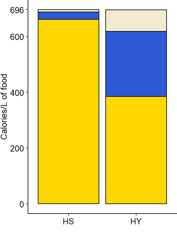
1.1.3 Figure 1C-D
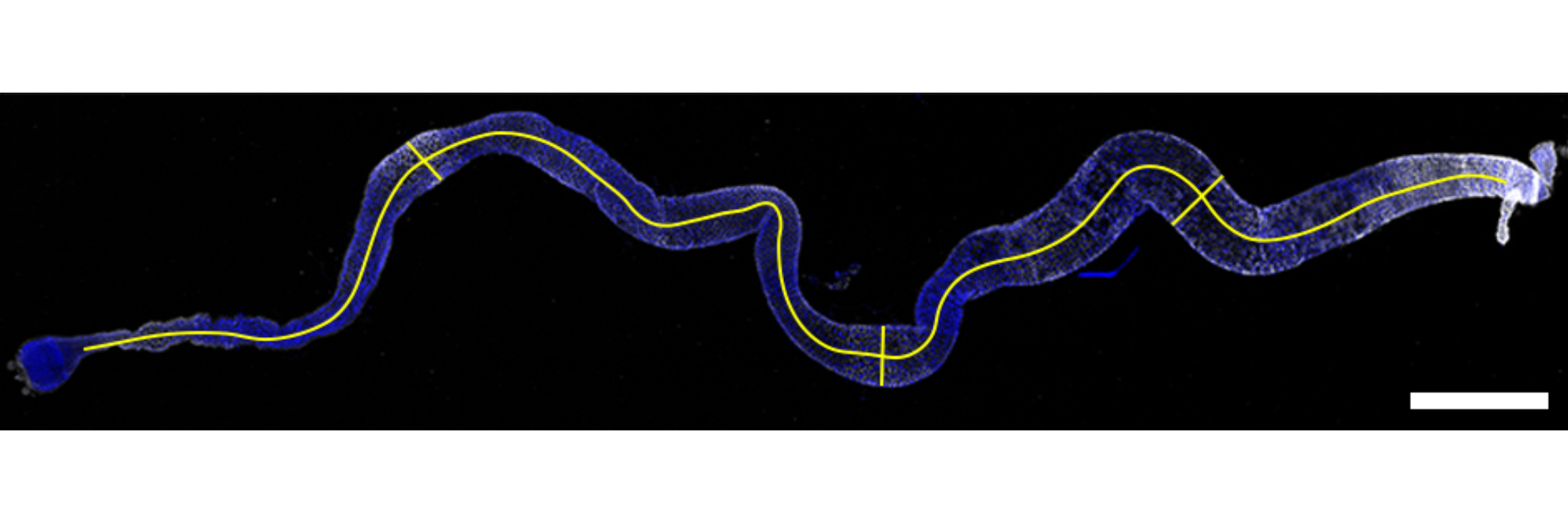
Canton S (Cs) flies fed on HS diet (C, first image) have shorter midguts than flies on HY (D, Second image). Complete graphical annotation can be found in manuscript figures

1.1.4 Figure 1E
Quantification of midgut length for HS vs HY at 5 days post eclosion.
Length_HSHY =
  d[["1E - 1S1A"]]%>%
  mutate_at(vars(starts_with("Total")),~./1000)%>%
  mutate_if(is.character,as.factor)%>%
  mutate_if(is.integer,as.factor)%>%
  dplyr::rename(Total_Length_mm=Total.L,
                Total_width_mm=Total.W,
                Day_of_treatment=Day)

Sample_size=
  Length_HSHY%>%
  group_by(Diet)%>%
  summarise(Sample_size=n())

Averages <- summarise(group_by(Length_HSHY, Diet), mean = mean(Total_Length_mm, na.rm = TRUE))

###Stats
mod.gen = fitme(log(Total_Length_mm) ~  Diet + (1 | Repeat), data = Length_HSHY)
shapiro.test(residuals(mod.gen))
    Shapiro-Wilk normality test

data:  residuals(mod.gen)
W = 0.98954, p-value = 0.9657bptest(log(Total_Length_mm) ~ Diet + (1 / Repeat), data = Length_HSHY)
    studentized Breusch-Pagan test

data:  log(Total_Length_mm) ~ Diet + (1/Repeat)
BP = 0.64174, df = 1, p-value = 0.4231
mod.gen1 = fitme(log(Total_Length_mm) ~ 1 + (1 | Repeat), data = Length_HSHY)
test = anova(mod.gen, mod.gen1)
Chi2_LRT_growth = 2*(mod.gen$APHLs[["p_v"]]-mod.gen1$APHLs[["p_v"]])
#Now we make a tab with the results
tab_stat = data.frame(Variable = as.character("HS vs HY"),
Rep = nlevels(Length_HSHY$Repeat),
chi2_LR = format(as.numeric(test$basicLRT$chi2_LR), digits = 2),
intercept = format(mod.gen$fixef[1],digits=3),
estimate = format(mod.gen$fixef[2],digits=3),
df = as.numeric(test$basicLRT$df),
Pvalue = as.numeric(format(pchisq(Chi2_LRT_growth,df=1,lower.tail = F),digits=2)))
tab_stat$sig = ifelse(tab_stat$Pvalue < 0.05 & tab_stat$Pvalue > 0.01, "*",
ifelse(tab_stat$Pvalue < 0.01 & tab_stat$Pvalue > 0.001, "**",
ifelse(tab_stat$Pvalue < 0.001, "***", "")))
tab_stat%>%
kable(col.names = c("Comparison", "Replicates", "Chi2","Intercept","Estimate","df" ,"p-value","Signif."),row.names = FALSE) %>%
add_header_above(c("log(Total_Length_mm) ~ Diet + (1 | Repeat)" = 8))%>%
kable_styling(bootstrap_options = c("striped", "hover", "condensed"), full_width = F)| Comparison | Replicates | Chi2 | Intercept | Estimate | df | p-value | Signif. |
|---|---|---|---|---|---|---|---|
| HS vs HY | 3 | 35 | 1.45 | 0.266 | 1 | 0 | *** |
### Plot
Limits = c("HS", "HY")
z= max(Length_HSHY$Total_Length_mm)
Plot_Fig1E=
  ggplot(Length_HSHY, aes(x = Diet, y = Total_Length_mm))+
  geom_violin(aes(fill = Diet), draw_quantiles = c(0.25, 0.5, 0.75), colour = "black", size = 0.2,adjust = 0.8) +
  geom_dotplot( colour = "black", fill = "white", binaxis = "y", stackdir = "center", binwidth = z/50) +
  geom_text(data = Sample_size, mapping = aes(x = Diet, y = 2.3, label = paste("(",Sample_size,")",sep="")),size=3)+
  geom_signif(annotation = formatC(paste("p=",tab_stat$Pvalue), digits = 2), textsize = 3, y_position = 7.3, xmin = 1, xmax = 2, tip_length = c(0.02, 0.02), vjust = -0.2)+
  scale_fill_manual(limits=Limits,
                    values=palette_diet_2)+
  scale_x_discrete("",
                   limits=c("HS", "HY"),
                   labels=c("HS", "HY"))+
  scale_y_continuous("Midgut length (mm)",
                     limits=c(2,8),
                     breaks=seq(2,8,by=1),
                     minor_breaks = seq(3, 7,by= 1))+
  stat_summary(fun = mean, geom = "point", size = 3, shape = 18, colour = "black", aes(group = Repeat)) +
  stat_summary(fun = mean, geom = "point", size = 2, shape = 18, aes(group = Repeat, colour = Repeat)) +
  scale_color_manual(values = palette_mean) +
  theme(aspect.ratio=2,
        panel.grid.major.y = element_line(colour = grey(0.45), linetype = "dashed", size = 0.2),
        panel.background = element_blank(),
        axis.title.x = element_text(size=Smallfont,colour="black"),
        axis.title.y = element_text(size=Smallfont,colour="black"),
        axis.line.x = element_line(colour="black",size=0.75),
        axis.line.y = element_line(colour="black",size=0.75),
        axis.ticks.x = element_line(size = 0.75),
        axis.ticks.y = element_line(size = 0.75),
        axis.text.x = element_text(size=Smallfont,colour="black"),
        axis.text.y = element_text(size=Smallfont,colour="black"),
        plot.margin = unit(Margin, "cm"),
        legend.direction = "vertical",
        legend.box = "horizontal",
        legend.position = "none",
        legend.key.height = unit(0.4, "cm"),
        legend.key.width= unit(0.6, "cm"),
        legend.title = element_text(face="italic",size=Smallfont),
        legend.key = element_rect(colour = 'white', fill = "white", linetype='dashed'),
        legend.text = element_text(size=SuperSmallfont),
        legend.background = element_rect(fill=NA))


#+
 # annotate("segment", x = 1, xend = 2, y = 7.2, yend = 7.2,
  #colour = "black", size =1.5)


Plot_Fig1E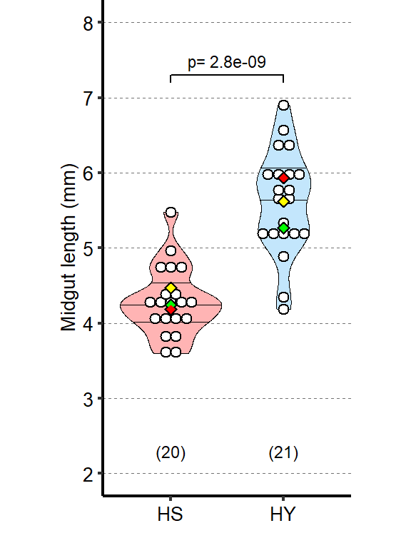
1.1.5 Figure 1F
Midgut length response to diet is strongly variable across the DGRP, with HY being generally longer than HS (i.e. the ratio length on HY/length on HS is between 1 and 1.4).
tab_GWAS_gut_mean =
  tab_GWAS_gut%>%
  group_by(dgrp_number,diet)%>%
  summarise(mean_gut_length=mean(totallength,na.rm=T))%>%
  spread(diet,mean_gut_length)%>%
  dplyr::rename(Mean_length_HS=x,
         Mean_length_HY=y)%>%
  mutate(Ratio = Mean_length_HY/Mean_length_HS)

tab_GWAS_gut_se =
  tab_GWAS_gut%>%
  group_by(dgrp_number,diet)%>%
  summarise(se_gut_length = se(totallength))%>%
  spread(diet,se_gut_length)%>%
  dplyr::rename(SE_length_HS=x,
         SE_length_HY=y)

tab_GWAS_gut_mean= left_join(tab_GWAS_gut_mean,tab_GWAS_gut_se)

colors=c("HS"="#FFB4B4","HY"="#C3E6FC","Ratio"="black")

plot_ratio_DGRP=
ggplot(tab_GWAS_gut_mean,aes(x = reorder(dgrp_number,Ratio))) +
  geom_point(aes(y=Mean_length_HS/1000,colour="HS"),stat="identity",size=0.7,shape=16)+
  geom_errorbar(aes(ymax = (Mean_length_HS+ SE_length_HS)/1000 , ymin = (Mean_length_HS - SE_length_HS)/1000 ,colour="HS"),width=0.1, show.legend=FALSE)+
  geom_point(aes(y=Mean_length_HY/1000,colour="HY"),stat="identity",size=0.7,shape=16)+
  geom_errorbar(aes(ymax = (Mean_length_HY+ SE_length_HY)/1000 , ymin = (Mean_length_HY - SE_length_HY)/1000 ,colour="HY"),width=0.1, show.legend=FALSE)+
  geom_point(aes(y=Ratio*3.9,colour="Ratio"),shape=17,size=0.7)+
  geom_hline(yintercept=3.9,linetype=2)+
  scale_y_continuous("Midgut length (mm)\n [mean \u00B1 se]",
                     limits=c(3,7.2),
                     sec.axis = sec_axis(~./3.9, name = "Ratio (HY/HS)", breaks = seq(0.8,1.8,0.2)))+
  scale_x_discrete("DGRP lines",expand=c(0.03,0.03))+
  scale_color_manual(values = colors )+
  theme(panel.background = element_blank(),
        (panel.border = element_blank()),
        axis.title.x = element_text(size=Smallfont,colour="black"),
        axis.title.y = element_text(size=Smallfont,colour="black"),
        axis.line.x = element_line(colour="black",size=0.75),
        axis.line.y = element_line(colour="black",size=0.75),
        axis.ticks.x = element_blank(),
        axis.ticks.y = element_line(size = 0.75),
        axis.text.x = element_blank(),
        axis.text.y = element_text(size=Smallfont,colour="black"),
        plot.margin = unit(Margin, "cm"),
        legend.direction = "horizontal",
        legend.box = "horizontal",
        legend.position = c(0.25,0.98),
        legend.key.height = unit(0.4, "cm"),
        legend.key.width= unit(0.4, "cm"),
        legend.title = element_blank(),
        legend.key = element_rect(colour = 'white', fill = "white", linetype='dashed'),
        legend.text = element_text(size=Smallfont),
        legend.background = element_rect(fill=NA))+
  guides(color=guide_legend(ncol=3))

plot_ratio_DGRP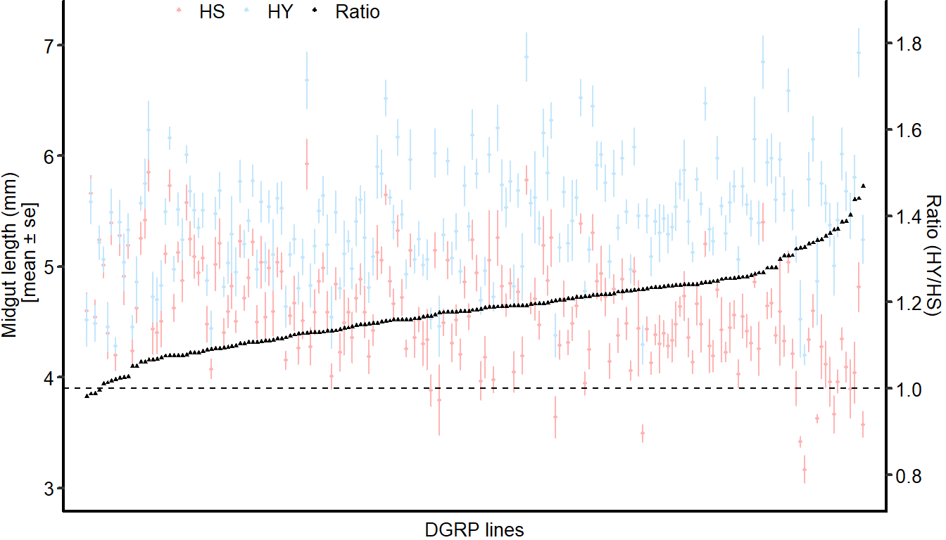
list_lines = unique(tab_GWAS_gut$dgrp_id)
Tab = NULL
for(i in list_lines){
  tmp= subset(tab_GWAS_gut,dgrp_id==i)
sample_size= tmp %>% group_by(diet)%>%summarize(n=n())

test= t.test(totallength~diet ,data=tmp)
Tab = rbind(Tab, c(i,test$parameter,test$statistic,test$p.value,test$estimate,sample_size[1,2],sample_size[2,2]))
}

colnames(Tab)=c("Line","df","t","Pvalue","Mean_HS","Mean_HY","Sample_size_HS","Sample_size_HY")
Tab = as.data.frame(Tab)%>%
  mutate(Pvalue=as.numeric(Pvalue),
         Mean_HS =as.numeric(Mean_HS),
         Mean_HY =as.numeric(Mean_HY),
         Difference = Mean_HY-Mean_HS )

Tab$Pv_adjust = p.adjust(Tab$Pvalue,method = "BH") # Here I control

length(which(Tab$Pv_adjust>0.05))
# 56 lines have no significant difference in size between diets
length(which(Tab$Pv_adjust<=0.05))
#132 lines have a significant difference in size between diets

Tab_sign = subset(Tab,Pv_adjust<=0.05)

length(which(Tab_sign$Difference<=0))
# 0 line was significantly smaller on HY

length(which(Tab_sign$Difference>0))
# 132 lines (i.e. all of those that were different) were significantly larger on HY
1.1.6 Figure 1G
Midgut re-sizing is allometric between regions of the midgut. Posterior midguts of flies fed HY exhibit a greater increase than anterior regions.
tab_GWAS_gut=
  tab_GWAS_gut%>%
  mutate(allometry=posteriorlength/anteriorlength)

tab_GWAS_gut_allometry_mean=
  tab_GWAS_gut%>%
  group_by(diet,dgrp_number)%>%
  summarise(mean_allometry=mean(allometry,na.rm=T))

Sample_size=
  tab_GWAS_gut_allometry_mean%>%
  group_by(diet)%>%
  summarise(Sample_size=n())

###Stats

mod.gen = fitme(mean_allometry ~  diet + (1 | dgrp_number) , data = tab_GWAS_gut_allometry_mean)
shapiro.test(residuals(mod.gen))
    Shapiro-Wilk normality test

data:  residuals(mod.gen)
W = 0.9809, p-value = 7.05e-05bptest(mean_allometry ~ diet + (1 / dgrp_number) , data = tab_GWAS_gut_allometry_mean)
    studentized Breusch-Pagan test

data:  mean_allometry ~ diet + (1/dgrp_number)
BP = 0.051149, df = 1, p-value = 0.8211
mod.gen1 = fitme(mean_allometry ~ 1 + (1 | dgrp_number), data = tab_GWAS_gut_allometry_mean)
test = anova(mod.gen, mod.gen1)
Chi2_LRT_growth = 2*(mod.gen$APHLs[["p_v"]]-mod.gen1$APHLs[["p_v"]])
#Now we make a tab with the results
tab_stat = data.frame(Variable = as.character(paste("HS vs HY")),
Rep = 1,
chi2_LR = round(as.numeric(test$basicLRT$chi2_LR), digits = 2),
intercept = format(mod.gen$fixef[1],digits=3),
estimate = format(mod.gen$fixef[2],digits=3),
df = as.numeric(test$basicLRT$df),
Pvalue = as.numeric(format(pchisq(Chi2_LRT_growth,df=1,lower.tail = F),digits=2)))
tab_stat$sig = ifelse(tab_stat$Pvalue < 0.05 & tab_stat$Pvalue > 0.01, "*",
ifelse(tab_stat$Pvalue < 0.01 & tab_stat$Pvalue > 0.001, "**",
ifelse(tab_stat$Pvalue < 0.001, "***", "")))
tab_stat%>%
kable(col.names = c("Comparison", "Replicates", "Chi2","Intercept","Estimate","df" ,"p-value","Signif."),row.names = FALSE) %>% add_header_above(c("mean_allometry ~ diet + (1 | dgrp_number)" = 8))%>%
kable_styling(bootstrap_options = c("striped", "hover", "condensed"), full_width = F)| Comparison | Replicates | Chi2 | Intercept | Estimate | df | p-value | Signif. |
|---|---|---|---|---|---|---|---|
| HS vs HY | 1 | 128.95 | 0.861 | 0.101 | 1 | 0 | *** |
### Plot

Plot_Fig1G=
  ggplot(tab_GWAS_gut_allometry_mean, aes(diet,mean_allometry, group=dgrp_number,color=diet)) +
  geom_path(size=0.3,color=grey(0.65))+
  geom_point(shape=16,size= 1)+
  scale_x_discrete("",
                   expand=c(0.1,0.1),
                   limits=c("x","y"),
                   labels=c("HS", "HY"))+
  scale_y_continuous("Posterior / anterior length",
                     limits=c(0.6, 1.4),
                     breaks=c(c(seq(0.5,1.4,by=0.1))))+
  scale_color_manual(limits=c("x","y"),
                    values=palette_diet_2)+
  annotate("text", label=paste("p=",tab_stat$Pvalue,sep=""), x= 1.5, y=1.4,size=3)+
  stat_summary(fun = mean, aes(group = 1),geom = "point", colour = "black", fill = "yellow", size = 3, shape = 23) +
  stat_summary(fun=mean, colour="black", geom="line", aes(group = 1),size=1,linetype=2)+
  theme(
    axis.title.x = element_text(size=Smallfont),
    axis.title.y = element_text(size=Smallfont),
    axis.line.x = element_line(colour="black",size=0.75),
    axis.line.y = element_line(colour="black",size=0.75),
    axis.ticks.x = element_line(size = 0.75),
    axis.ticks.y = element_line(size = 0.75),
    axis.text.x = element_text(size=Smallfont,colour="black"),
    axis.text.y = element_text(size=Smallfont,colour="black"),
    legend.position = "none",
    panel.background = element_blank())

Plot_Fig1G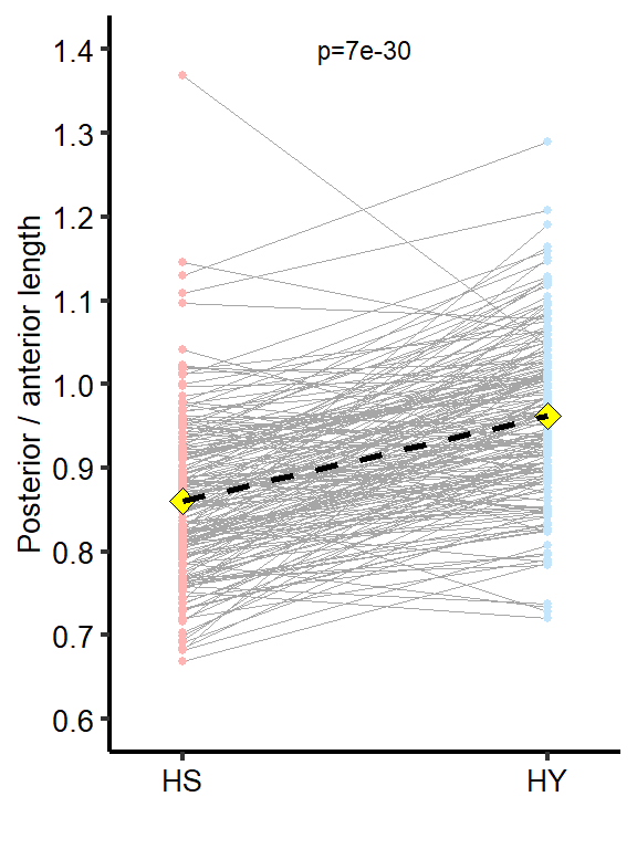
##Export Figure 1
1.2 Figure 1 - figure supplement 1
1.2.1 Figure 1S1A
Canton S (Cs) flies fed HS diet have narrower midguts than those fed HY diet. Width was measured in three point along the gut (Region 2, 3 and 4, as visible in the yellow annotation in Figure 1C,D) and the sum of these three measurement was used as proxy for midgut width. Measurements are from the same guts as in Figure 1E
Length_HSHY =
  d[["1E - 1S1A"]]%>%
  mutate_at(vars(starts_with("Total")),~./1000)%>%
  mutate_if(is.character,as.factor)%>%
  mutate_if(is.integer,as.factor)%>%
  dplyr::rename(Total_Length_mm=Total.L,
         Total_width_mm=Total.W,
         Day_of_treatment=Day)

Sample_size=
  Length_HSHY%>%
  group_by(Diet)%>%
  summarise(Sample_size=n())

###Stats

mod.gen = fitme(log(Total_width_mm) ~  Diet + (1 | Repeat), data = Length_HSHY)
shapiro.test(residuals(mod.gen))
    Shapiro-Wilk normality test

data:  residuals(mod.gen)
W = 0.95797, p-value = 0.1335bptest(log(Total_width_mm) ~ Diet + (1 / Repeat), data = Length_HSHY)
    studentized Breusch-Pagan test

data:  log(Total_width_mm) ~ Diet + (1/Repeat)
BP = 0.17388, df = 1, p-value = 0.6767
mod.gen1 = fitme(log(Total_width_mm) ~ 1 + (1 | Repeat), data = Length_HSHY)
test = anova(mod.gen, mod.gen1)
Chi2_LRT_growth = 2*(mod.gen$APHLs[["p_v"]]-mod.gen1$APHLs[["p_v"]])
#Now we make a tab with the results
tab_stat = data.frame(Variable = as.character(paste("HS vs HY")),
Rep = nlevels(Length_HSHY$Repeat),
chi2_LR = round(as.numeric(test$basicLRT$chi2_LR), digits = 2),
intercept = format(mod.gen$fixef[1],digits=3),
estimate = format(mod.gen$fixef[2],digits=3),
df = as.numeric(test$basicLRT$df),
Pvalue = as.numeric(format(pchisq(Chi2_LRT_growth,df=1,lower.tail = F),digits=2)))
tab_stat$sig = ifelse(tab_stat$Pvalue < 0.05 & tab_stat$Pvalue > 0.01, "*",
ifelse(tab_stat$Pvalue < 0.01 & tab_stat$Pvalue > 0.001, "**",
ifelse(tab_stat$Pvalue < 0.001, "***", "")))
tab_stat%>%
kable(col.names = c("Comparison", "Replicates", "Chi2","Intercept","Estimate","df" ,"p-value","Signif."),row.names = FALSE) %>%
add_header_above(c("log(Total_width_mm) ~ Diet + (1 | Repeat)" = 8))%>%
kable_styling(bootstrap_options = c("striped", "hover", "condensed"), full_width = F)| Comparison | Replicates | Chi2 | Intercept | Estimate | df | p-value | Signif. |
|---|---|---|---|---|---|---|---|
| HS vs HY | 3 | 55.48 | -0.754 | 0.374 | 1 | 0 | *** |
### Plot
Limits = c("HS", "HY")
z = max(Length_HSHY$Total_width_mm)

Plot_Fig1S1A=
ggplot(Length_HSHY, aes(x = Diet, y = Total_width_mm))+
  geom_violin(aes(fill = Diet), draw_quantiles = c(0.25, 0.5, 0.75), colour = "black", size = 0.2,adjust = 0.6) +
  geom_dotplot( colour = "black", fill = "white", binaxis = "y", stackdir = "center", binwidth = z/50) +
  geom_text(data = Sample_size, mapping = aes(x = Diet, y = 0.25, label = paste("(",Sample_size,")",sep="")),size=3)+
  geom_signif(annotation = formatC(paste("p=",tab_stat$Pvalue), digits = 2), textsize = 3, y_position = 0.93, xmin = 1, xmax = 2, tip_length = c(0.02, 0.02), vjust = -0.2)+
  scale_fill_manual(limits=Limits,
                    values=palette_diet_2)+
  scale_x_discrete("",
                   limits=c("HS", "HY"),
                   breaks=c("HS", "HY"))+
  scale_y_continuous("Midgut width (mm)",
                     limits=c(0.2,1),
                     breaks=seq(0.2,1,by=0.1))+
  stat_summary(fun = mean, geom = "point", size = 3, shape = 18,colour = "black",aes(group=Repeat)) +
  stat_summary(fun = mean, geom = "point", size = 2, shape = 18,aes(group=Repeat, colour = Repeat)) +
  scale_color_manual(values=palette_mean)+
  theme(panel.background = element_blank(),
        panel.grid.major.y = element_line(colour = grey(0.45), linetype = "dashed", size = 0.2),
                axis.title.x = element_text(size=Smallfont,colour="black"),
                axis.title.y = element_text(size=Smallfont,colour="black"),
                axis.line.x = element_line(colour="black",size=0.75),
                axis.line.y = element_line(colour="black",size=0.75),
                axis.ticks.x = element_line(size = 0.75),
                axis.ticks.y = element_line(size = 0.75),
                axis.text.x = element_text(size=Smallfont,colour="black"),
                axis.text.y = element_text(size=Smallfont,colour="black"),
                plot.margin = unit(Margin, "cm"),
                legend.direction = "vertical",
                legend.box = "horizontal",
                legend.position = "none",
                legend.key.height = unit(0.4, "cm"),
                legend.key.width= unit(0.6, "cm"),
                legend.title = element_text(face="italic",size=Smallfont),
                legend.key = element_rect(colour = 'white', fill = "white", linetype='dashed'),
                legend.text = element_text(size=SuperSmallfont),
                legend.background = element_rect(fill=NA))

Plot_Fig1S1A
1.2.2 Figure 1S1B
Length of midguts on HY diet is similar to standard diets used in the field (Bloomington [Bl] cornmeal and Bl molasses).
tab_stddiets_rev =
  d[["1 - S1B"]]%>%
  mutate(Total_Length_mm =Total.L/1000)%>%
  mutate_if(is.character,as.factor)%>%
  mutate_if(is.integer,as.factor)%>%
  mutate(Sugar=fct_relevel(Diet,"HS","HY", "BL Cornmeal", "BL Molasses"))

Sample_size=
  tab_stddiets_rev%>%
  group_by(Diet)%>%
  summarise(Sample_size=n())

###Stats

mod.gen = fitme((Total_Length_mm) ~  Diet + (1 | Repeat), data = tab_stddiets_rev)
shapiro.test(residuals(mod.gen))
    Shapiro-Wilk normality test

data:  residuals(mod.gen)
W = 0.96479, p-value = 0.00686bptest((Total_Length_mm) ~ Diet + (1 / Repeat), data = tab_stddiets_rev)
    studentized Breusch-Pagan test

data:  (Total_Length_mm) ~ Diet + (1/Repeat)
BP = 1.7773, df = 3, p-value = 0.6199
mod.gen1 = fitme((Total_Length_mm) ~ 1 + (1 | Repeat), data = tab_stddiets_rev)
test = anova(mod.gen, mod.gen1)
Chi2_LRT_growth = 2*(mod.gen$APHLs[["p_v"]]-mod.gen1$APHLs[["p_v"]])
#Now we make a tab with the results
tab_stat = data.frame(Variable = as.character(paste("Anova diets")),
Rep = nlevels(tab_stddiets_rev$Repeat),
chi2_LR = round(as.numeric(test$basicLRT$chi2_LR), digits = 2),
intercept = format(mod.gen$fixef[1],digits=3),
estimate = format(mod.gen$fixef[2],digits=3),
df = as.numeric(test$basicLRT$df),
Pvalue = as.numeric(format(pchisq(Chi2_LRT_growth,df=1,lower.tail = F),digits=2)))
tab_stat$sig = ifelse(tab_stat$Pvalue < 0.05 & tab_stat$Pvalue > 0.01, "*",
ifelse(tab_stat$Pvalue < 0.01 & tab_stat$Pvalue > 0.001, "**",
ifelse(tab_stat$Pvalue < 0.001, "***", "")))
tab_stat%>%
kable(col.names = c("Comparison", "Replicates", "Chi2","Intercept","Estimate","df" ,"p-value","Signif."),row.names = FALSE) %>% add_header_above(c("(Total_Length_mm) ~ Diet + (1 | Repeat)" = 8))%>%
kable_styling(bootstrap_options = c("striped", "hover", "condensed"), full_width = F)| Comparison | Replicates | Chi2 | Intercept | Estimate | df | p-value | Signif. |
|---|---|---|---|---|---|---|---|
| Anova diets | 3 | 53.44 | 5.07 | 0.435 | 3 | 0 | *** |
mod.gen = lmer(Total_Length_mm ~  Diet + (1 | Repeat), data = tab_stddiets_rev)
multcomp = glht(mod.gen, linfct=mcp(Diet="Tukey"))
tmp = cld(multcomp)

letter_position = aggregate(data=tab_stddiets_rev,Total_Length_mm ~ Diet, max)

tab_letter =  as.data.frame(tmp$mcletters$Letters)
tab_letter$Diet=rownames(tab_letter)
colnames(tab_letter)[1] = "Letter"
tab_letter = left_join(tab_letter,letter_position)

Limits =c("HS","HY", "BL Cornmeal", "BL Molasses")
Labels =c("HS","HY", "Bl cornmeal", "Bl molasses")
cbbPalette = c("#FFB4B4","#C3E6FC", "#f6efe5", "#f6efe5")

z = max(tab_stddiets_rev$Total_Length_mm, na.rm = TRUE)

Plot_Fig1S1B=
  ggplot(tab_stddiets_rev, aes(x = Diet, y = Total_Length_mm))+
  geom_violin(aes(fill = Diet), draw_quantiles = c(0.25, 0.5, 0.75), colour = "black", size = 0.2,adjust = 0.8, alpha = 0.5) +
  geom_dotplot( colour = "black", fill = "white", binaxis = "y", stackdir = "center", binwidth = z/35) +
  geom_text(data = Sample_size, mapping = aes(x = Diet, y = 1.8, label = paste("(",Sample_size,")",sep="")),size=3)+
  geom_text(data = tab_stat, mapping = aes(x = 2.5, y = 7.5, label = paste("p=",format(Pvalue,digits=2))),size=3)+
  geom_text(data = tab_letter, mapping = aes(x = Diet, y = Total_Length_mm+0.6, label = Letter),size=3)+
  scale_fill_manual(limits=Limits,
                    values=cbbPalette)+
  scale_x_discrete("",
                   limits=Limits,
                   labels=Labels)+
  scale_y_continuous("Midgut length (mm)",
                     limits=c(1.6,8),
                     breaks=seq(2,7,by=1))+
   stat_summary(fun = mean, geom = "point", size = 3, shape = 18, colour = "black", aes(group = Repeat)) +
                     stat_summary(fun = mean, geom = "point", size = 2, shape = 18, aes(group = Repeat, colour = Repeat)) +
                     scale_color_manual(values = palette_mean) +
  theme(panel.background = element_blank(),
        panel.grid.major.y = element_line(colour = grey(0.45), linetype = "dashed", size = 0.2),
        axis.title.x = element_text(size=Smallfont,colour="black"),
        axis.title.y = element_text(size=Smallfont,colour="black"),
        axis.line.x = element_line(colour="black",size=0.75),
        axis.line.y = element_line(colour="black",size=0.75),
        axis.ticks.x = element_line(size = 0.75),
        axis.ticks.y = element_line(size = 0.75),
        axis.text.x = element_text(size=Smallfont,colour="black"),
        axis.text.y = element_text(size=Smallfont,colour="black"),
        plot.margin = unit(c(0,0,0,0.5), "cm"),
        legend.direction = "vertical",
        legend.box = "horizontal",
        legend.position = "none",
        legend.key.height = unit(0.4, "cm"),
        legend.key.width= unit(0.6, "cm"),
        legend.title = element_text(face="italic",size=Smallfont),
        legend.key = element_rect(colour = 'white', fill = "white", linetype='dashed'),
        legend.text = element_text(size=SuperSmallfont),
        legend.background = element_rect(fill=NA))

Plot_Fig1S1B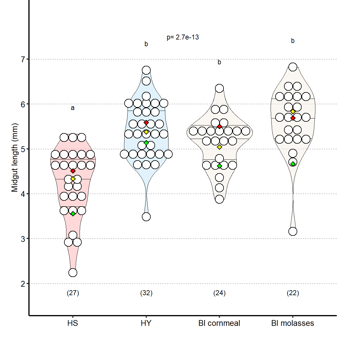
1.2.3 Figure 1S1C
Un-mated females and mated males have lower response to diet compared to mated female flies. Statistics: comparison of the interaction between diet and mating status/sex. Full annotation on figure present in manuscript
tab_MUmM_rev =
  d[["1 - S1C"]]%>%
  mutate_at(vars(!starts_with("Total")),as.factor)%>%
  mutate(Total_Length_mm=Total.L/1000)%>%
  mutate(Treatment=fct_relevel(Treatment,c("Mated females","Un-mated females","Males")))

Sample_size=
  tab_MUmM_rev%>%
  group_by(Diet,Treatment)%>%
  summarise(Sample_size=n())

###Stats
#Un-mated
tmp = subset(tab_MUmM_rev, Treatment%in%c("Mated females","Un-mated females"))
mod.gen = fitme((Total_Length_mm) ~  Diet * Treatment + (1 | Repeat),data = tmp)
shapiro.test(residuals(mod.gen))
    Shapiro-Wilk normality test

data:  residuals(mod.gen)
W = 0.98312, p-value = 0.2426bptest((Total_Length_mm) ~ Diet + Treatment + (1 / Repeat),data = tmp)
    studentized Breusch-Pagan test

data:  (Total_Length_mm) ~ Diet + Treatment + (1/Repeat)
BP = 0.27838, df = 2, p-value = 0.8701
mod.gen1 = fitme((Total_Length_mm) ~ Diet + Treatment + (1 | Repeat),data = tmp)
test = anova(mod.gen, mod.gen1)
Chi2_LRT_growth = 2*(mod.gen$APHLs[["p_v"]]-mod.gen1$APHLs[["p_v"]])
tab_stat = data.frame(Treatment = as.character(paste("Mated vs Un-mated females")),
Rep = nlevels(tmp$Repeat),
chi2_LR = round(as.numeric(test$basicLRT$chi2_LR), digits = 2),
intercept = format(mod.gen$fixef[1],digits=3),
estimate = format(mod.gen$fixef[2],digits=3),
df = as.numeric(test$basicLRT$df),
Pvalue = as.numeric(format(pchisq(Chi2_LRT_growth,df=1,lower.tail = F),digits=1,scientific=F)))
tab_stat_Un_mated=tab_stat
#Male
tmp = subset(tab_MUmM_rev, Treatment%in%c("Mated females","Males"))
mod.gen = fitme(log(Total_Length_mm) ~ Diet * Treatment + (1 | Repeat),data = tmp)
shapiro.test(residuals(mod.gen))
    Shapiro-Wilk normality test

data:  residuals(mod.gen)
W = 0.97901, p-value = 0.115bptest(log(Total_Length_mm) ~ Diet + Treatment + (1 / Repeat),data = tmp)
    studentized Breusch-Pagan test

data:  log(Total_Length_mm) ~ Diet + Treatment + (1/Repeat)
BP = 6.2807, df = 2, p-value = 0.04327
mod.gen1 = fitme(log(Total_Length_mm) ~ Diet + Treatment + (1 | Repeat),data = tmp)
test = anova(mod.gen, mod.gen1)
Chi2_LRT_growth = 2*(mod.gen$APHLs[["p_v"]]-mod.gen1$APHLs[["p_v"]])
tab_stat = data.frame(Treatment = as.character(paste("Mated vs Males")),
Rep = nlevels(tmp$Repeat),
chi2_LR = round(as.numeric(test$basicLRT$chi2_LR), digits = 2),
intercept = format(mod.gen$fixef[1],digits=3),
estimate = format(mod.gen$fixef[2],digits=3),
df = as.numeric(test$basicLRT$df),
Pvalue = as.numeric(format(pchisq(Chi2_LRT_growth,df=1,lower.tail = F),digits=1,scientific=F)))
tab_stat_Male=tab_stat
tab_stat=rbind(tab_stat_Male,tab_stat_Un_mated)
tab_stat$sig = ifelse(tab_stat$Pvalue < 0.05 & tab_stat$Pvalue > 0.009, "*", #changed to 0.009 because Un-mated is exactle 0.01
ifelse(tab_stat$Pvalue < 0.01 & tab_stat$Pvalue > 0.001, "**",
ifelse(tab_stat$Pvalue < 0.001, "***", "")))
tab_stat%>%
kable(col.names = c("Variable", "Replicates", "Chi2","Intercept","Estimate","df" ,"p-value","Signif."),row.names = FALSE) %>%
add_header_above(c("log(Total_Length_mm) ~ Diet + Treatment + Diet : Treatment + (1 | Repeat)" = 8))%>%
kable_styling(bootstrap_options = c("striped", "hover", "condensed"), full_width = F)| Variable | Replicates | Chi2 | Intercept | Estimate | df | p-value | Signif. |
|---|---|---|---|---|---|---|---|
| Mated vs Males | 3 | 23.35 | 1.46 | 0.229 | 1 | 1e-06 | *** |
| Mated vs Un-mated females | 3 | 6.57 | 4.35 | 1.11 | 1 | 1e-02 |
|
tab_stat$Treatment = as.factor(tab_stat$Treatment)
tab
Error in eval(expr, envir, enclos): objet 'tab' introuvable### Plot
tab_stat_1S1C=tab_stat
Plot_Fig1S1C=
ggplot(tab_MUmM_rev, aes(x = Diet, y = Total_Length_mm))+
geom_violin(aes(fill = Diet), draw_quantiles = c(0.25, 0.5, 0.75), colour = "black", size = 0.2,adjust = 0.8) +
geom_dotplot( colour = "black", fill = "white", binaxis = "y", stackdir = "center", binwidth = 0.15) +
geom_text(data = Sample_size, mapping = aes(x = Diet, y = 1.7, label = paste("(",Sample_size,")",sep="")),size=3)+
facet_grid(.~ Treatment)+
scale_fill_manual(values=palette_diet_2)+
scale_x_discrete("",
limits=c("HS","HY"),
labels=c("HS","HY"))+
scale_y_continuous("Midgut length (mm)",
limits=c(1.5,8),
breaks=seq(2,6,by=1))+
stat_summary(fun = mean, geom = "point", size = 3, shape = 18, colour = "black", aes(group = Repeat)) +
stat_summary(fun = mean, geom = "point", size = 2, shape = 18, aes(group = Repeat, colour = Repeat)) +
stat_summary(fun = mean, colour = "black", geom = "line", aes(group = Repeat)) +
scale_color_manual(values = palette_mean) +
theme(panel.grid.major.y = element_line(colour = grey(0.45), linetype = "dashed", size = 0.2),
panel.background = element_blank(),
axis.title.x = element_text(size=Smallfont,colour="black"),
axis.title.y = element_text(size=Smallfont,colour="black"),
axis.line.x = element_line(colour="black",size=0.75),
axis.line.y = element_line(colour="black",size=0.75),
axis.ticks.x = element_line(size = 0.75),
axis.ticks.y = element_line(size = 0.75),
axis.text.x = element_text(size=Smallfont,colour="black"),
axis.text.y = element_text(size=Smallfont,colour="black"),
plot.margin = unit(Margin, "cm"),
legend.direction = "vertical",
legend.box = "horizontal",
legend.position = "none",
legend.key.height = unit(0.4, "cm"),
legend.key.width= unit(0.6, "cm"),
legend.title = element_text(face="italic",size=Smallfont),
legend.key = element_rect(colour = 'white', fill = "white", linetype='dashed'),
legend.text = element_text(size=SuperSmallfont),
legend.background = element_rect(fill=NA),
strip.text.x = element_text(size = Smallfont, colour = "black", margin = margin(t = 2, r = 0, b = 2, l = 0)),
strip.text.y = element_text(size = Smallfont, colour = "black", margin = margin(t = 2, r = 0, b = 2, l = 0)),
strip.background = element_rect(fill=NA, colour="black"),
strip.placement="outside")
Plot_Fig1S1C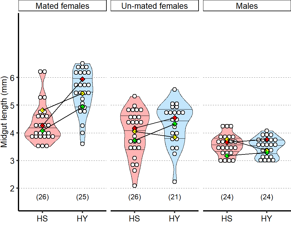
1.2.4 Figure 1S1D
Feeding assay shows higher dietary intake on HS than on HY diet. Absorbance measured after 1 day of assay, each day along a 5-day period from eclosion, for a total of 5 times per condition/repeat
Tab_absorbance =
  d[["1 - S1D"]]%>%
  mutate_if(is.character,as.factor)%>%
  mutate_if(is.integer,as.factor)%>%
  dplyr::rename(Diet=Food)

Sample_size=
  Tab_absorbance%>%
  group_by(Diet)%>%
  summarise(Sample_size=n())

###Stats

mod.gen = fitme(Absorbance ~  Diet + (1 | Repeat), data = Tab_absorbance)
shapiro.test(residuals(mod.gen))
    Shapiro-Wilk normality test

data:  residuals(mod.gen)
W = 0.91089, p-value = 0.01567bptest(Absorbance ~ Diet + (1 / Repeat), data = Tab_absorbance)
    studentized Breusch-Pagan test

data:  Absorbance ~ Diet + (1/Repeat)
BP = 5.6989, df = 1, p-value = 0.01698
mod.gen1 = fitme(Absorbance ~ 1 + (1 | Repeat), data = Tab_absorbance)
test = anova(mod.gen, mod.gen1)
Chi2_LRT_growth = 2*(mod.gen$APHLs[["p_v"]]-mod.gen1$APHLs[["p_v"]])
#Now we make a tab with the results
tab_stat = data.frame(Variable = as.character(paste("HS vs HY")),
Rep = nlevels(Tab_absorbance$Repeat),
chi2_LR = round(as.numeric(test$basicLRT$chi2_LR), digits = 2),
intercept = format(mod.gen$fixef[1],digits=3),
estimate = format(mod.gen$fixef[2],digits=3),
df = as.numeric(test$basicLRT$df),
Pvalue = as.numeric(format(pchisq(Chi2_LRT_growth,df=1,lower.tail = F),digits=2)))
tab_stat$sig = ifelse(tab_stat$Pvalue < 0.05 & tab_stat$Pvalue > 0.01, "*",
ifelse(tab_stat$Pvalue < 0.01 & tab_stat$Pvalue > 0.001, "**",
ifelse(tab_stat$Pvalue < 0.001, "***", "")))
tab_stat%>%
kable(col.names = c("Comparison", "Replicates", "Chi2","Intercept","Estimate","df" ,"p-value","Signif."),row.names = FALSE) %>% add_header_above(c("Absorbance ~ Diet + (1 | Repeat)" = 8))%>%
kable_styling(bootstrap_options = c("striped", "hover", "condensed"), full_width = F)| Comparison | Replicates | Chi2 | Intercept | Estimate | df | p-value | Signif. |
|---|---|---|---|---|---|---|---|
| HS vs HY | 3 | 30.71 | 0.404 | -0.256 | 1 | 0 | *** |
##Plot
Limits = c("HS", "HY")
z = max(Tab_absorbance$Absorbance)

Plot_Fig1S1D=
ggplot(Tab_absorbance, aes(x = Diet, y = Absorbance))+
  geom_violin(aes(fill = Diet), draw_quantiles = c(0.25, 0.5, 0.75), colour = "black", size = 0.2,adjust = 0.8) +
  geom_dotplot( colour = "black", fill = "white", binaxis = "y", stackdir = "center", binwidth = z/40) +
  geom_text(data = Sample_size, mapping = aes(x = Diet, y = 0.02, label = paste("(",Sample_size,")",sep="")),size=3)+
  geom_signif(annotation = formatC(paste("p=",tab_stat$Pvalue), digits = 2), textsize = 3, y_position = 0.58, xmin = 1, xmax = 2, tip_length = c(0.02, 0.02), vjust = -0.2)+

  scale_fill_manual(limits=Limits,
                    values=palette_diet_2)+
  scale_x_discrete("",
                   limits=c("HS", "HY"),
                   breaks=c("HS", "HY"))+
  scale_y_continuous("Absorbance",
                     limits=c(0,0.6),
                     breaks=seq(0,0.5,by=0.1))+
  stat_summary(fun = mean, geom = "point", size = 3, shape = 18,colour = "black",aes(group=Repeat)) +
  stat_summary(fun = mean, geom = "point", size = 2, shape = 18,aes(group=Repeat, colour = Repeat)) +
  scale_color_manual(values=palette_mean)+
  theme(panel.background = element_blank(),
        panel.grid.major.y = element_line(colour = grey(0.45), linetype = "dashed", size = 0.2),
                axis.title.x = element_text(size=Smallfont,colour="black"),
                axis.title.y = element_text(size=Smallfont,colour="black"),
                axis.line.x = element_line(colour="black",size=0.75),
                axis.line.y = element_line(colour="black",size=0.75),
                axis.ticks.x = element_line(size = 0.75),
                axis.ticks.y = element_line(size = 0.75),
                axis.text.x = element_text(size=Smallfont,colour="black"),
                axis.text.y = element_text(size=Smallfont,colour="black"),
                plot.margin = unit(Margin, "cm"),
                legend.direction = "vertical",
                legend.box = "horizontal",
                legend.position = "none",
                legend.key.height = unit(0.4, "cm"),
                legend.key.width= unit(0.6, "cm"),
                legend.title = element_text(face="italic",size=Smallfont),
                legend.key = element_rect(colour = 'white', fill = "white", linetype='dashed'),
                legend.text = element_text(size=SuperSmallfont),
                legend.background = element_rect(fill=NA))

Plot_Fig1S1D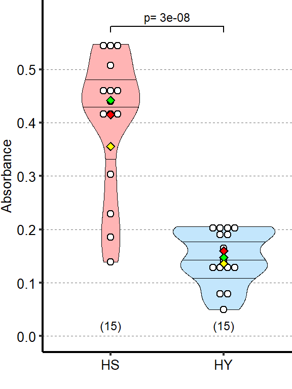
1.2.5 Figure 1S1E
Microbes are not required for the difference in size observed between HS and HY fed flies. Germ-free flies exhibit similar diet-induced increase in size as conventionally reared flies at both 7- and 14-days post eclosion (statistics: comparison of the interaction between diets and conv. reared/germ free treatment). Of note, at 7-days post eclosion we observed longer guts in germ free flies compared to conventionally reared flies (significant on HS diet). This difference was lost at 14-days post eclosion (Post hoc Tukey test from GLMM summarized by letter at the bottom of chart). Full statistical annotation on figure present in manuscript
Length_HSHY_germfree =
  d[["1 - S1E"]]%>%
  mutate_at(vars(starts_with("Total")),~./1000)%>%
  mutate_if(is.character,as.factor)%>%
  mutate_if(is.integer,as.factor)%>%
  dplyr::rename(Total_Length_mm=Total.L,
         Day_of_treatment=Day)


Sample_size=
  Length_HSHY_germfree%>%
  group_by(Diet,Treatment, Day_of_treatment)%>%
  summarise(Sample_size=n())

Sample_size$Sample_size <- as.numeric(Sample_size$Sample_size)


###Stats Day 7 interaction
Length_HSHY_germfree_Day7 = subset(Length_HSHY_germfree, Day_of_treatment == "7")
mod.gen = fitme(log(Total_Length_mm) ~  Diet + Treatment + Diet : Treatment + (1 | Repeat), data = Length_HSHY_germfree_Day7)
shapiro.test(residuals(mod.gen))
    Shapiro-Wilk normality test

data:  residuals(mod.gen)
W = 0.98828, p-value = 0.5513bptest(log(Total_Length_mm) ~ Diet + Treatment + (1 / Repeat), data = Length_HSHY_germfree_Day7)
    studentized Breusch-Pagan test

data:  log(Total_Length_mm) ~ Diet + Treatment + (1/Repeat)
BP = 5.3166, df = 2, p-value = 0.07007
mod.gen1 = fitme(log(Total_Length_mm) ~ Diet + Treatment + (1 | Repeat), data = Length_HSHY_germfree_Day7)
test = anova(mod.gen, mod.gen1)
Chi2_LRT_growth = 2*(mod.gen$APHLs[["p_v"]]-mod.gen1$APHLs[["p_v"]])
#Now we make a tab with the results
tab_stat7 = data.frame(Variable = as.character(paste("Response to diet Day7")),
Rep = as.numeric(nlevels(Length_HSHY_germfree_Day7$Repeat)),
chi2_LR = round(as.numeric(test$basicLRT$chi2_LR), digits = 2),
intercept = format(mod.gen$fixef[1],digits=3),
estimate = format(mod.gen$fixef[4],digits=3),
df = as.numeric(test$basicLRT$df),
Pvalue = as.numeric(format(pchisq(Chi2_LRT_growth,df=1,lower.tail = F),digits=2)))
tab_stat7$sig = ifelse(tab_stat7$Pvalue < 0.05 & tab_stat7$Pvalue > 0.01, "*",
ifelse(tab_stat7$Pvalue < 0.01 & tab_stat7$Pvalue > 0.001, "**",
ifelse(tab_stat7$Pvalue < 0.001, "***", "")))
tab_stat7%>%
kable(col.names = c("Response to diet Day7", "Replicates", "Chi2","Intercept","Estimate","df" ,"p-value","Signif."),row.names = FALSE) %>% add_header_above(c("log(Total_Length_mm) ~ Diet + Treatment + Diet : Treatment + (1 | Repeat)" = 8))%>%
kable_styling(bootstrap_options = c("striped", "hover", "condensed"), full_width = F)| Response to diet Day7 | Replicates | Chi2 | Intercept | Estimate | df | p-value | Signif. |
|---|---|---|---|---|---|---|---|
| Response to diet Day7 | 3 | 0.15 | 1.35 | -0.015 | 1 | 0.7 |
tab_stat_int_GF7=tab_stat7


###Stats Day 14 interaction
Length_HSHY_germfree_Day14 = subset(Length_HSHY_germfree, Day_of_treatment == "14")
mod.gen = fitme(log(Total_Length_mm) ~  Diet + Treatment + Diet : Treatment + (1 | Repeat), data = Length_HSHY_germfree_Day14)
shapiro.test(residuals(mod.gen))
    Shapiro-Wilk normality test

data:  residuals(mod.gen)
W = 0.98625, p-value = 0.4111bptest(log(Total_Length_mm) ~ Diet + Treatment + (1 / Repeat), data = Length_HSHY_germfree_Day14)
    studentized Breusch-Pagan test

data:  log(Total_Length_mm) ~ Diet + Treatment + (1/Repeat)
BP = 0.62752, df = 2, p-value = 0.7307
mod.gen1 = fitme(log(Total_Length_mm) ~ Diet + Treatment + (1 | Repeat), data = Length_HSHY_germfree_Day14)
test = anova(mod.gen, mod.gen1)
Chi2_LRT_growth = 2*(mod.gen$APHLs[["p_v"]]-mod.gen1$APHLs[["p_v"]])
#Now we make a tab with the results
tab_stat14 = data.frame(Variable = as.character(paste("Response to diet Day14")),
Rep = as.numeric(nlevels(Length_HSHY_germfree_Day14$Repeat)),
chi2_LR = round(as.numeric(test$basicLRT$chi2_LR), digits = 2),
intercept = format(mod.gen$fixef[1],digits=3),
estimate = format(mod.gen$fixef[4],digits=3),
df = as.numeric(test$basicLRT$df),
Pvalue = as.numeric(format(pchisq(Chi2_LRT_growth,df=1,lower.tail = F),digits=2)))
tab_stat14$sig = ifelse(tab_stat14$Pvalue < 0.05 & tab_stat14$Pvalue > 0.01, "*",
ifelse(tab_stat14$Pvalue < 0.01 & tab_stat14$Pvalue > 0.001, "**",
ifelse(tab_stat14$Pvalue < 0.001, "***", "")))
tab_stat14%>%
kable(col.names = c("Response to diet Day14", "Replicates", "Chi2","Intercept","Estimate","df" ,"p-value","Signif."),row.names = FALSE) %>% add_header_above(c("log(Total_Length_mm) ~ Diet + Treatment + Diet : Treatment + (1 | Repeat)" = 8))%>%
kable_styling(bootstrap_options = c("striped", "hover", "condensed"), full_width = F)| Response to diet Day14 | Replicates | Chi2 | Intercept | Estimate | df | p-value | Signif. |
|---|---|---|---|---|---|---|---|
| Response to diet Day14 | 3 | 3.75 | 1.29 | -0.0976 | 1 | 0.053 |
tab_stat_int_GF14=tab_stat14


#Model including all samples and Post HOC test

Length_HSHY_germfree$Treat_Diet_Day = as.factor(paste(Length_HSHY_germfree$Treatment, Length_HSHY_germfree$Diet, Length_HSHY_germfree$Day_of_treatment, sep="_"))


mod.gen = lmer(log(Total_Length_mm) ~ Treat_Diet_Day + (1 | Repeat), data = Length_HSHY_germfree)

shapiro.test(residuals(mod.gen))
    Shapiro-Wilk normality test

data:  residuals(mod.gen)
W = 0.99294, p-value = 0.4774bptest(log(Total_Length_mm) ~ Treat_Diet_Day + (1/ Repeat), data = Length_HSHY_germfree)
    studentized Breusch-Pagan test

data:  log(Total_Length_mm) ~ Treat_Diet_Day + (1/Repeat)
BP = 16.062, df = 7, p-value = 0.02455
multcomp = glht(mod.gen, linfct=mcp(Treat_Diet_Day="Tukey"))
tmp = cld(multcomp)
letter_position = aggregate(data=Length_HSHY_germfree,Total_Length_mm ~ Treat_Diet_Day, min)
tab_letter = as.data.frame(tmp$mcletters$Letters)
tab_letter$Treat_Diet_Day=rownames(tab_letter)
colnames(tab_letter)[1] = "Letter"
tab_letter = left_join(tab_letter,letter_position)
tab_letter$Treat_Diet_Day= as.factor(tab_letter$Treat_Diet_Day)
tab_letter$Day_of_treatment = as.factor(mid(tab_letter$Treat_Diet_Day,7, 2))
tab_letter$Diet = as.factor(mid(tab_letter$Treat_Diet_Day, 4,2))
tab_letter$Treatment = as.factor(left(tab_letter$Treat_Diet_Day, 2))
### Plot
Limits = c("HS", "HY")
z= max(Length_HSHY_germfree$Total_Length_mm)
Treatment.status = c("Conv. reared", "Germ free")
names(Treatment.status) = c("CR", "GF")
Plot_Fig1S1E=
ggplot(Length_HSHY_germfree, aes(x = Diet, y = Total_Length_mm))+
geom_violin(aes(fill = Diet), draw_quantiles = c(0.25, 0.5, 0.75), colour = "black", size = 0.2,adjust = 0.8) +
geom_dotplot( colour = "black", fill = "white", binaxis = "y", stackdir = "center", binwidth = z/50) +
geom_text(data = tab_letter, mapping = aes(x = Diet, y = Total_Length_mm-0.4, label = Letter),size=3)+
facet_wrap(Day_of_treatment~Treatment,labeller=labeller(Treatment=Treatment.status), nrow = 1)+
geom_text(data = Sample_size, mapping = aes(x = Diet, y = 1.35, label = paste("(",Sample_size,")",sep="")),size=3)+
scale_fill_manual(limits=Limits,
values=palette_diet_2)+
scale_x_discrete("",
limits=c("HS", "HY"),
breaks=c("HS", "HY"))+
scale_y_continuous("Midgut length (mm)",
limits=c(1,8),
breaks=seq(2,8,by=1))+
stat_summary(fun = mean, geom = "point", size = 3, shape = 18,colour = "black",aes(group=Repeat)) +
stat_summary(fun = mean, geom = "point", size = 2, shape = 18,aes(group=Repeat, colour = Repeat)) +
stat_summary(fun=mean, colour="black", geom="line",aes(group=Repeat))+
scale_color_manual(values=palette_mean)+
theme(panel.background = element_blank(),
panel.grid.major.y = element_line(colour = grey(0.45), linetype = "dashed", size = 0.2),
axis.title.x = element_text(size=Smallfont,colour="black"),
axis.title.y = element_text(size=Smallfont,colour="black"),
axis.line.x = element_line(colour="black",size=0.75),
axis.line.y = element_line(colour="black",size=0.75),
axis.ticks.x = element_line(size = 0.75),
axis.ticks.y = element_line(size = 0.75),
axis.text.x = element_text(size=Smallfont,colour="black"),
axis.text.y = element_text(size=Smallfont,colour="black"),
plot.margin = unit(Margin, "cm"),
legend.direction = "vertical",
legend.box = "horizontal",
legend.position = "none",
legend.key.height = unit(0.4, "cm"),
legend.key.width= unit(0.6, "cm"),
legend.title = element_text(face="italic",size=Smallfont),
legend.key = element_rect(colour = 'white', fill = "white", linetype='dashed'),
legend.text = element_text(size=SuperSmallfont),
legend.background = element_rect(fill=NA),
strip.text.x = element_text(size =Smallfont, colour = "black", margin = margin(t = 2, r = 0, b = 2, l = 0)),
strip.text.y = element_text(size =Smallfont, colour = "black", margin = margin(t = 2, r = 0, b = 2, l = 0)),
strip.background = element_rect(fill=NA, colour="black"),
strip.placement="outside")
Plot_Fig1S1E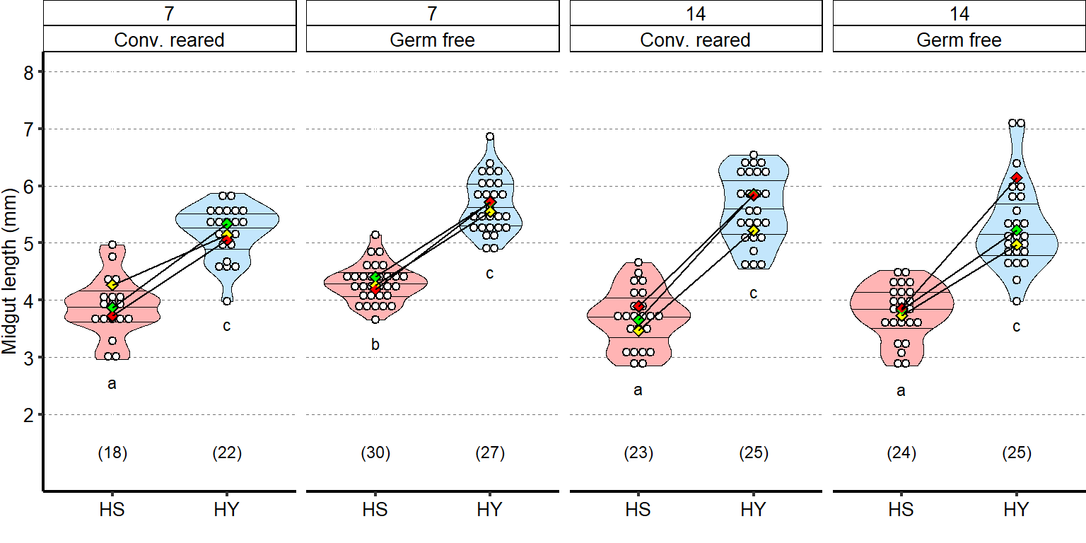
##Export Figure S1
1.3 Figure 1 - figure supplement 2
1.3.1 Figure 1S2A
Scheme depicting regional organization of the gut. The gut comprises three main anatomical regions: foregut (comprising the crop), midgut and hindgut. The midgut itself can be divided in anterior (blue), middle (green) and posterior (purple). Additional subregions have been described (Buchon et al., 2013; Marianes and Spradling, 2013).
 img1S2A = readImage("F:/Dropbox/Github/Bonfini_eLife_2021/data/1- S2A.jpg")
 gob_imageFig1S2A = rasterGrob(img1S2A)
 grid.draw(gob_imageFig1S2A)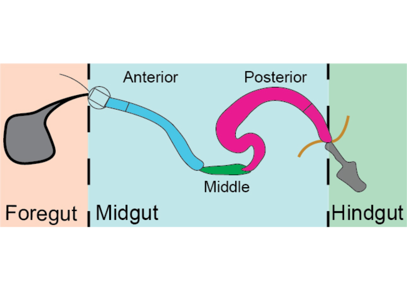
1.3.2 Figure 1S2B
All regions of the midgut (x-axis) respond variably to diet composition, but the response of the posterior midgut length more closely reflects the response of the total midgut length. Red lines represent linear regression and black dashed lines are the lines of equivalence.
tab_GWAS_gut$dgrpDiet = factor(paste(tab_GWAS_gut$dgrp_id, tab_GWAS_gut$diet), ordered=T)

meansMat = aggregate(as.matrix(tab_GWAS_gut[,c("anteriorlength", "middlelength", "posteriorlength",  "totallength")]) ~ diet * dgrp_id, tab_GWAS_gut, mean)
rownames(meansMat) = paste(meansMat$dgrp_id, meansMat$diet, sep="_")
colnames(meansMat) <- c("diet","dgrp_id", "Anterior Length", "Middle Length", "Posterior Length", "Total Length")
meansMatX = subset(meansMat, diet=="x")
meansMatY = subset(meansMat, diet=="y")
all(meansMatX$dgrp_id == meansMatY$dgrp_id)
meansMatX = meansMatX[,!colnames(meansMatX) %in% c("dgrp_id", "diet")]
meansMatY = meansMatY[,!colnames(meansMatY) %in% c("dgrp_id", "diet")]

meansMatY=
meansMatY %>%
  setNames(str_to_sentence(names(.)))

meansMatX=
meansMatX %>%
  setNames(str_to_sentence(names(.)))

RIs <- meansMatY / meansMatX
RIs <- RIs[,!grepl("width", colnames(RIs))]
plotRegress <- function(x,y, datRange, textCex, ...){
    regn <- lm(y ~ x)
    plot(y ~ x, xlim=datRange, ylim=datRange, ...)
    abline(a=0,b=1, col=alpha(1, 0.5), lty=2)
    abline(a=coef(regn)[1], b=coef(regn)[2],col=2)

    val=round(summary(regn)$adj.r.squared, 1)
    text(y=max(datRange), x=min(datRange),
    labels=bquote(R^2 ~"="~ .(val)), adj=0, cex=textCex)

    text(y=max(datRange) - (0.1 * diff(range(RIs))), x=min(datRange),
    labels=paste("p =", signif(summary(regn)$coefficients[2,4], 2)), adj=0, cex=textCex)

    text(y=max(datRange) - (0.2 * diff(range(RIs))), x=min(datRange),
    labels=paste("y = ", signif(coef(regn)[2], 2), "x", " + ", signif(coef(regn)[1], 2), sep=""), adj=0, cex=textCex)
}

jpeg(filename =  "Plot_Fig1S2B.jpeg",
      res = 300,
      width = 9, height = 3, units = 'in' )

 par(bty="n", mfrow=c(1,3), cex.main=1.4, cex.lab=1.4, cex.axis=1.4)

for(i in 1:3){
 plotRegress(x=RIs[,i], y=RIs[,4], xlab=paste(c("Anterior", "Middle", "Posterior")[i], "HY length / HS length"), ylab="Total HY length / HS length", bty="n", cex=0.75, pch=16, datRange=range(RIs), las=1, asp =1, textCex=1.4)
 }

dev.off()
img1S2B = readImage("F:/Dropbox/Github/Bonfini_eLife_2021/data/Plot_Fig1S2B.jpeg")
gob_imageFig1S2B = rasterGrob(img1S2B)
grid.draw(gob_imageFig1S2B)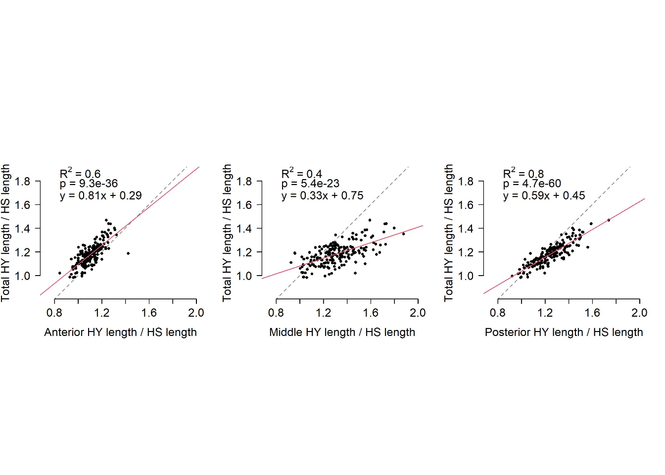
##Export Figure 1S2
1.4 Figure 1 - figure supplement 3
1.4.1 Figure 1S3A
Variation in impact of diet on midgut length in the DGRP maps to genes with functions connected to epithelial turnover. The Manhattan plot summarizes the p-value per chromosomal locus (grey bars) associated with GWAS analysis. Highlighted genes have been selected based on their statistical significance, their function, and the effect of the genetic variation (e.g. non-synonymous mutation, etc.).
img1S3A = readImage("F:/Dropbox/Github/Bonfini_eLife_2021/data/1 - S3.jpg")
gob_imageFig1S3A = rasterGrob(img1S3A)
grid.draw(gob_imageFig1S3A)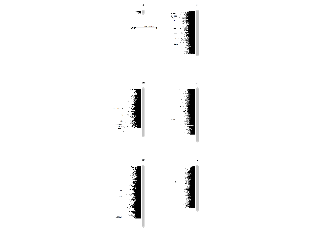
##Export Figure
2 Figure 2. Sugar antagonizes yeast-induced increase of midgut length
2.1 Figure 2 - main
2.1.1 Figure 2A
Midgut length is maximized at specific points in diet space. Adult flies were maintained for 5 days from eclosion on one of 28 diets based on different caloric concentration and yeast to sucrose ratios (see figure 1-figure supplement 1A for scheme on diets used and sample size). The list of recipes can be found in Table1. The figure shows contours of a thin-plate spline (Generalized Additive Model) of length (mm, coded by colors) as a function of yeast and sucrose in diet. Colored dots represent mean of samples in a particular diet.
tab_nutri_geo =
  d[["2A"]]%>%
    mutate(Total.Lmm = Total.L / 1000)

tab_nutri_geo$YSdiet <- with(tab_nutri_geo, (Yeast.in.Diet)/(Sucrose.in.Diet))
    tab_nutri_geo$YSingested <- with(tab_nutri_geo, (Yeast.ingested)/(Sucrose.ingested))

jpeg(filename =  "F:/Dropbox/Github/Bonfini_eLife_2021/data/Plot_Fig2A.jpeg",
     res = 600,
     width = 5, height = 4, units = 'in' )
par(cex=1, mar = c(4.5, 4.5, 1, 3))
with(tab_nutri_geo, geomPlotta(x = Sucrose.in.Diet, y = Yeast.in.Diet, z = Total.Lmm, alf = 1, xlim = c(-10, 300), ylim = c(-10, 300), xlab = "Sucrose in diet (g/L)", ylab = "Yeast in diet (g/L)", frame.plot= FALSE, cex.lab=1.2, cex.axis =1, las=1, labcex=1, asp=1))
img2A = readImage("F:/Dropbox/Github/Bonfini_eLife_2021/data/Plot_Fig2A.jpeg")
gob_imageFig2A = rasterGrob(img2A)
grid.draw(gob_imageFig2A)
2.1.2 Figure 2B
Plot show an increase in midgut length with increased amount of yeast ingested.
tab_nutri_geo =
  d[["2A"]]%>%
    mutate(Total.Lmm = Total.L / 1000)

tab_nutri_geo$title1 <- "Midgut length vs yeast ingested"

graph2 <- ggplot(tab_nutri_geo, aes(x=Yeast.ingested, y=Total.Lmm))

Plot_Fig2B=
  graph2 + geom_point(size=2,shape=16) + geom_smooth(span=1, size=1, color = "blue") +
  scale_y_continuous("Midgut length (mm)") +
  scale_x_continuous("Yeast ingested (g/L x absorbance)") +
    theme(panel.background = element_blank(),
        panel.grid.major.y = element_line(colour = grey(0.45), linetype = "dashed", size = 0.2),
        axis.title.x = element_text(size=Smallfont,colour="black"),
        axis.title.y = element_text(size=Smallfont,colour="black"),
        axis.line.x = element_line(colour="black",size=0.75),
        axis.line.y = element_line(colour="black",size=0.75),
        axis.ticks.x = element_line(size = 0.75),
        axis.ticks.y = element_line(size = 0.75),
        axis.text.x = element_text(size=Smallfont,colour="black"),
        axis.text.y = element_text(size=Smallfont,colour="black"),
        plot.margin = unit(Margin, "cm"))

Plot_Fig2B
2.1.3 Figure 2C
Plots show a decrease in midgut length with increased amount of sucrose ingested.
tab_nutri_geo =
  d[["2A"]]%>%
    mutate(Total.Lmm = Total.L / 1000)

graph3 <- ggplot(tab_nutri_geo, aes(x=Sucrose.ingested, y=Total.Lmm))

Plot_Fig2C=
  graph3 + geom_point(size=2,shape=16) + geom_smooth(span=1, size=1, color = "red")+
  scale_y_continuous("Midgut length (mm)") +
  scale_x_continuous("Sucrose ingested (g/L x absorbance)") +
  theme(panel.background = element_blank(),
        panel.grid.major.y = element_line(colour = grey(0.45), linetype = "dashed", size = 0.2),
        axis.title.x = element_text(size=Smallfont,colour="black"),
        axis.title.y = element_text(size=Smallfont,colour="black"),
        axis.line.x = element_line(colour="black",size=0.75),
        axis.line.y = element_line(colour="black",size=0.75),
        axis.ticks.x = element_line(size = 0.75),
        axis.ticks.y = element_line(size = 0.75),
        axis.text.x = element_text(size=Smallfont,colour="black"),
        axis.text.y = element_text(size=Smallfont,colour="black"),
        plot.margin = unit(Margin, "cm"))

Plot_Fig2C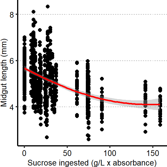
2.1.4 Figure 2D
Plot show an increase in midgut length with ratio of yeast to sucrose ingested.
tab_nutri_geo =
  d[["2A"]]%>%
    mutate(Total.Lmm = Total.L / 1000)

graph4 <- ggplot(tab_nutri_geo, aes(x=(Yeast.ingested/Sucrose.ingested), y=Total.Lmm))

Plot_Fig2D=

graph4 + geom_point(size=2,shape=16) + geom_smooth(span=1, size=1, color = "green")+
  scale_y_continuous("Midgut length (mm)") +
  scale_x_continuous("Y:S ingested") +
  theme(panel.background = element_blank(),
        panel.grid.major.y = element_line(colour = grey(0.45), linetype = "dashed", size = 0.2),
        axis.title.x = element_text(size=Smallfont,colour="black"),
        axis.title.y = element_text(size=Smallfont,colour="black"),
        axis.line.x = element_line(colour="black",size=0.75),
        axis.line.y = element_line(colour="black",size=0.75),
        axis.ticks.x = element_line(size = 0.75),
        axis.ticks.y = element_line(size = 0.75),
        axis.text.x = element_text(size=Smallfont,colour="black"),
        axis.text.y = element_text(size=Smallfont,colour="black"),
        plot.margin = unit(Margin, "cm"))

Plot_Fig2D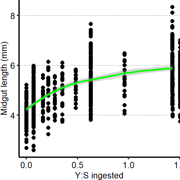
2.1.5 Figure 2E
Several nutrients from yeast (proteins, lipids, vitamins/minerals) are required to increase midgut length. Nutrients from yeast (proteins, amino acids, lipids, cholesterol, vitamins/minerals) were added against a base diet of only the amount of sucrose found in HY and devoid of yeast. Letters above violin plots represent grouping by statistical differences (Post hoc Tukey on GLMM). Bars beneath the main plot describe caloric content provided by the different components. Proper label annotation (in line with the chart) can be found in manuscript figures
tab_lenght_complement =
  d[["2E"]]%>%
  mutate_if(is.character,as.factor)%>%
  mutate_if(is.integer,as.factor)%>%
  dplyr::rename(Diet=Food,
        Total_Length_mm = Total.Lmm)

tab_lenght_complement$Diet = factor(tab_lenght_complement$Diet, levels = c("HS",
"S74Y0 (A)",
"A+Cas2",
"A+Cas4",
"A+AA",
"A+AA2",
"A+L4",
"A+Ch0.4",
"A+L2+Ch0.2",
"A+L4+Ch0.4",
"A+V2",
"A+V4",
"A+C4+L4+Ch0.4",
"A+C4+L4+Ch0.4+V2",
"HY")) #Order Diets

Sample_size=
  tab_lenght_complement%>%
  group_by(Diet)%>%
  summarise(Sample_size=n())

###Stats

mod.gen = fitme(log(Total_Length_mm) ~  Diet + (1 | Repeat), data = tab_lenght_complement)
shapiro.test(residuals(mod.gen))
    Shapiro-Wilk normality test

data:  residuals(mod.gen)
W = 0.99393, p-value = 0.1361bptest(log(Total_Length_mm) ~ Diet + (1 / Repeat), data = tab_lenght_complement)
    studentized Breusch-Pagan test

data:  log(Total_Length_mm) ~ Diet + (1/Repeat)
BP = 41.593, df = 14, p-value = 0.0001434
mod.gen1 = fitme(log(Total_Length_mm) ~ 1 + (1 | Repeat), data = tab_lenght_complement)
test = anova(mod.gen, mod.gen1)
Chi2_LRT_growth = 2*(mod.gen$APHLs[["p_v"]]-mod.gen1$APHLs[["p_v"]])
#Now we make a tab with the results
tab_stat = data.frame(Variable = as.character(paste("Anova diets")),
Rep = nlevels(tab_lenght_complement$Repeat),
chi2_LR = round(as.numeric(test$basicLRT$chi2_LR), digits = 2),
intercept = format(mod.gen$fixef[1],digits=3),
estimate = format(mod.gen$fixef[2],digits=3),
df = as.numeric(test$basicLRT$df),
Pvalue = as.numeric(format(pchisq(Chi2_LRT_growth,df=1,lower.tail = F),digits=2)))
tab_stat$sig = ifelse(tab_stat$Pvalue < 0.05 & tab_stat$Pvalue > 0.01, "*",
ifelse(tab_stat$Pvalue < 0.01 & tab_stat$Pvalue > 0.001, "**",
ifelse(tab_stat$Pvalue < 0.001, "***", "")))
tab_stat%>%
kable(col.names = c("Comparison", "Replicates", "Chi2","Intercept","Estimate","df" ,"p-value","Signif."),row.names = FALSE) %>% add_header_above(c("log(Total_Length_mm) ~ Diet + (1 | Repeat)" = 8))%>%
kable_styling(bootstrap_options = c("striped", "hover", "condensed"), full_width = F)| Comparison | Replicates | Chi2 | Intercept | Estimate | df | p-value | Signif. |
|---|---|---|---|---|---|---|---|
| Anova diets | 3 | 313.48 | 1.45 | -0.0461 | 14 | 0 | *** |
mod.gen = lmer(Total_Length_mm ~  Diet + (1 | Repeat), data = tab_lenght_complement)
multcomp = glht(mod.gen, linfct=mcp(Diet="Tukey"))

tmp = cld(multcomp)

letter_position = aggregate(data=tab_lenght_complement,Total_Length_mm ~ Diet, max)

tab_letter =  as.data.frame(tmp$mcletters$Letters)
tab_letter$Diet=rownames(tab_letter)
colnames(tab_letter)[1] = "Letter"
tab_letter = left_join(tab_letter,letter_position)

### Plot

Limits= c("HS", "S74Y0 (A)", "A+Cas2", "A+Cas4", "A+AA", "A+AA2", "A+L4", "A+Ch0.4", "A+L2+Ch0.2", "A+L4+Ch0.4", "A+V2", "A+V4", "A+C4+L4+Ch0.4","A+C4+L4+Ch0.4+V2", "HY")

cbbPalette = c("#FFB4B4", "#f6efe5", "#f6efe5", "#f6efe5", "#f6efe5", "#f6efe5", "#f6efe5", "#f6efe5", "#f6efe5", "#f6efe5", "#f6efe5", "#f6efe5", "#f6efe5", "#f6efe5", "#C3E6FC")


z = max(tab_lenght_complement$Total_Length_mm, na.rm=TRUE)

Plot_Fig2E=
  ggplot(tab_lenght_complement, aes(x = Diet, y = Total_Length_mm))+
  geom_violin(aes(fill = Diet), draw_quantiles = c(0.25, 0.5, 0.75), colour = "black", size = 0.2,adjust = 0.8) +
  geom_dotplot( colour = "black", fill = "white", binaxis = "y", stackdir = "center", binwidth = z / 60) +
  geom_text(data = Sample_size, mapping = aes(x = Diet, y = 2.2, label = paste("(",Sample_size,")",sep="")),size=3)+
  geom_text(data = tab_letter, mapping = aes(x = Diet, y = Total_Length_mm+0.4, label = Letter),size=3)+
  geom_text(data = tab_stat, mapping = aes(x = 2, y = 7.5, label = paste("p=",Pvalue)),size=3)+
  scale_fill_manual(limits=Limits,
                    values=cbbPalette)+
  scale_x_discrete("",
                   limits=Limits)+
  scale_y_continuous("Midgut length (mm)",
                     limits=c(2,8),
                     breaks=seq(3,7,by=1))+
                     stat_summary(fun = mean, geom = "point", size = 2, shape = 18, colour = "black", aes(group = Repeat)) +
                     stat_summary(fun = mean, geom = "point", size = 1, shape = 18, aes(group = Repeat, colour = Repeat)) +
                     scale_color_manual(values = palette_mean) +
  theme(panel.background = element_blank(),
        panel.grid.major.y = element_line(colour = grey(0.45), linetype = "dashed", size = 0.2),
        axis.title.x = element_blank(),
        axis.title.y = element_text(size=Smallfont,colour="black"),
        axis.line.x = element_line(colour="black",size=0.75),
        axis.line.y = element_line(colour="black",size=0.75),
        axis.ticks.x = element_line(size = 0.75),
        axis.ticks.y = element_line(size = 0.75),
        axis.text.x = element_blank(),
        axis.text.y = element_text(size=Smallfont,colour="black"),
        plot.margin = unit(c(0,0,0,0.5), "cm"),
        legend.direction = "vertical",
        legend.box = "horizontal",
        legend.position = "none",
        legend.key.height = unit(0.4, "cm"),
        legend.key.width= unit(0.5, "cm"),
        legend.title = element_text(face="italic",size=Smallfont),
        legend.key = element_rect(colour = 'white', fill = "white", linetype='dashed'),
        legend.text = element_text(size=SuperSmallfont),
        legend.background = element_rect(fill=NA))

tab_component_calories= mutate_if(d[["2E - calories"]],is.character,as.factor)
tab_component_calories$Component <- factor(tab_component_calories$Component, levels = c("Lipids", "Proteins", "Carbohydrates"))

Limits_2 = c("Lipids","Proteins","Carbohydrates")
Labels = c("Lipids","Proteins","Carbohydrates")

Plot_Fig2E_bis=
ggplot(tab_component_calories,aes(x=Diet,y=Calories.contributed))+
geom_bar(stat="identity",aes(fill=Component),color="black",width=.90)+
  scale_fill_manual(limits=Limits_2,
                      values=palette_component_3,
                      labels=Labels)+
  scale_x_discrete("",
                     limits=Limits)+
  scale_y_reverse("Calories",
                     breaks=c(seq(0,1400,by=300)))+
  theme(axis.title.x = element_blank(),
        axis.title.y =  element_text(size=Smallfont,colour="black"),
        axis.line.x = element_line(colour="white"),
        axis.line.y = element_line(colour="black"),
        axis.ticks.x = element_line(colour="white"),
        axis.ticks.y = element_line(),
        axis.text.x = element_blank(),
        axis.text.y = element_text(size=Smallfont,colour="black"),
        panel.grid = element_blank(),
        plot.margin = unit(c(0,0,0,0), "cm"),
        legend.direction = "horizontal",
        legend.box = "horizontal",
        legend.position = "bottom",
        legend.margin=margin(t=0.1, r=0.2, b=0.1, l=0, unit="cm"),
        legend.title = element_blank(),
        legend.key = element_rect(colour = 'white', fill = "white", linetype='dashed'),
        legend.text = element_text(size=Smallfont),
        legend.background = element_rect(fill="white", colour="black"),
        legend.key.size = unit(0.5,"cm"),

        strip.text.x = element_text(size =Mediumfont, colour = "black",face="italic"),
        strip.text.y = element_text(size =Mediumfont, colour = "black",face="italic"),
        strip.background = element_rect(fill=NA, colour="black"),
        strip.placement="outside",
        panel.background = element_rect(fill="transparent"))+
  guides(fill=guide_legend(ncol=3))


plot_2E = grid.arrange(Plot_Fig2E,
                       Plot_Fig2E_bis+ theme(legend.position="none"),
                       grid.text("HS",x=0.15, y=0.2, just="left",gp = gpar(fontsize=Smallfont,fontface="bold")),
                       grid.text("HY",x=0.95, y=1, just="left",gp = gpar(fontsize=Smallfont,fontface="bold")),
                       grid.text("Sucrose in HY completed with:",x=0.21, y=0.9,just="left",gp = gpar(fontsize=Smallfont,fontface="bold")),
                       grid.text("Casein       x0  x2  x4                                            x4 x4", x=0.02, y=0.52,just="left",gp = gpar(fontsize=Smallfont,fontface="bold")),
                       grid.text("AAs            x0            x1 x2", x=0.02, y=0.51,just="left",gp = gpar(fontsize=Smallfont,fontface="bold")),

                       grid.text("Lard           x0                       x4       x2 x4            x4  x4", x=0.02, y=0.50,just="left",gp = gpar(fontsize=Smallfont,fontface="bold")),
                       grid.text("Chol.          x0                            x1  x1 x1            x1  x1", x=0.02, y=0.49,just="left",gp = gpar(fontsize=Smallfont,fontface="bold")),

                       grid.text("Vit.             x0                                            x2  x4       x2", x=0.02, y=0.48,just="left",gp = gpar(fontsize=Smallfont,fontface="bold")),

                       ncol = 1, heights = c(2,1,0.2,0.15, 0.15,0.15,0.15,0.15,0.15,0.2))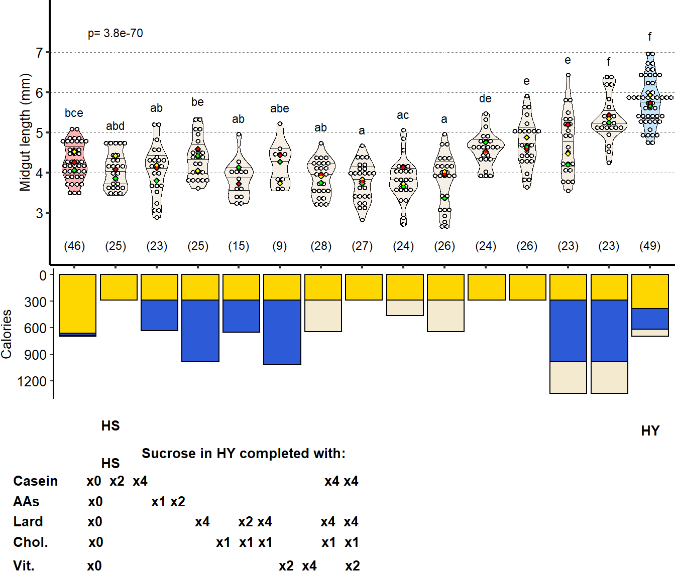
2.1.6 Figure 2F
Midgut size is antagonized by sugar, but not other added calories. Diet with only lipids, isocaloric with HS and HY diets, results in midguts of lengths comparable to those on HS diet. Substitution of sucrose from HS diet with isocaloric lipids (Lipids HS) results in midguts as long as those on HY. Midguts of flies reared on a diet substituting sucrose in HY diet with lipids (Lipids HY) are also similar in length to those of flies fed HY. Letters above violin plots represent grouping by statistical differences (Post hoc Tukey on GLMM). Bottom part of the chart (bar graph) describes caloric content provided by the different components.
tab_lipids =
  d[["2F"]]%>%
  mutate(Total_Length_mm =Total.L/1000)%>%
  mutate_if(is.character,as.factor)%>%
  mutate_if(is.integer,as.factor)%>%
  dplyr::rename(Diet=Food)

Sample_size=
  tab_lipids%>%
  group_by(Diet)%>%
  summarise(Sample_size=n())

###Stats

mod.gen = fitme(log(Total_Length_mm) ~  Diet + (1 | Repeat), data = tab_lipids)
shapiro.test(residuals(mod.gen))
    Shapiro-Wilk normality test

data:  residuals(mod.gen)
W = 0.98586, p-value = 0.2715bptest(log(Total_Length_mm) ~ Diet + (1 / Repeat), data = tab_lipids)
    studentized Breusch-Pagan test

data:  log(Total_Length_mm) ~ Diet + (1/Repeat)
BP = 6.0006, df = 4, p-value = 0.1991
mod.gen1 = fitme(log(Total_Length_mm) ~ 1 + (1 | Repeat), data = tab_lipids)
test = anova(mod.gen, mod.gen1)
Chi2_LRT_growth = 2*(mod.gen$APHLs[["p_v"]]-mod.gen1$APHLs[["p_v"]])
#Now we make a tab with the results
tab_stat = data.frame(Variable = as.character(paste("Anova diets")),
Rep = nlevels(tab_lipids$Repeat),
chi2_LR = round(as.numeric(test$basicLRT$chi2_LR), digits = 2),
intercept = format(mod.gen$fixef[1],digits=3),
estimate = format(mod.gen$fixef[2],digits=3),
df = as.numeric(test$basicLRT$df),
Pvalue = as.numeric(format(pchisq(Chi2_LRT_growth,df=1,lower.tail = F),digits=2)))
tab_stat$sig = ifelse(tab_stat$Pvalue < 0.05 & tab_stat$Pvalue > 0.01, "*",
ifelse(tab_stat$Pvalue < 0.01 & tab_stat$Pvalue > 0.001, "**",
ifelse(tab_stat$Pvalue < 0.001, "***", "")))
tab_stat%>%
kable(col.names = c("Comparison", "Replicates", "Chi2","Intercept","Estimate","df" ,"p-value","Signif."),row.names = FALSE) %>% add_header_above(c("log(Total_Length_mm) ~ Diet + (1 | Repeat)" = 8))%>%
kable_styling(bootstrap_options = c("striped", "hover", "condensed"), full_width = F)| Comparison | Replicates | Chi2 | Intercept | Estimate | df | p-value | Signif. |
|---|---|---|---|---|---|---|---|
| Anova diets | 3 | 112.99 | 1.59 | 0.224 | 4 | 0 | *** |
mod.gen = lmer(Total_Length_mm ~  Diet + (1 | Repeat), data = tab_lipids)
multcomp = glht(mod.gen, linfct=mcp(Diet="Tukey"))
tmp = cld(multcomp)

letter_position = aggregate(data=tab_lipids,Total_Length_mm ~ Diet, max)

tab_letter =  as.data.frame(tmp$mcletters$Letters)
tab_letter$Diet=rownames(tab_letter)
colnames(tab_letter)[1] = "Letter"
tab_letter = left_join(tab_letter,letter_position)

Limits =c("Lard Only","HS","HS Lard sub","HY Lard sub","HY")
Labels =c("Yeast:Lipid 0:1","Yeast:Sugar 1:14 (HS)","Yeast:Lipid 1:14","Yeast:Lipid 1:0.7","Yeast:Sugar 1:0.7 (HY)")
cbbPalette = c("#f6efe5", "#FFB4B4", "#f6efe5", "#f6efe5", "#C3E6FC")

z = max(tab_lipids$Total_Length_mm, na.rm = TRUE)

Plot_Fig2F=
  ggplot(tab_lipids, aes(x = Diet, y = Total_Length_mm))+
  geom_violin(aes(fill = Diet), draw_quantiles = c(0.25, 0.5, 0.75), colour = "black", size = 0.2,adjust = 0.8, alpha = 0.5) +
  geom_dotplot( colour = "black", fill = "white", binaxis = "y", stackdir = "center", binwidth = z/60) +
  geom_text(data = Sample_size, mapping = aes(x = Diet, y = 2.5, label = paste("(",Sample_size,")",sep="")),size=3)+
  geom_text(data = tab_stat, mapping = aes(x = 1.7, y = 7.5, label = paste("p=",format(Pvalue,digits=2))),size=3)+
  geom_text(data = tab_letter, mapping = aes(x = Diet, y = Total_Length_mm+0.4, label = Letter),size=3)+
  scale_fill_manual(limits=Limits,
                    values=cbbPalette)+
  scale_x_discrete("",
                   limits=Limits,
                   labels=Labels)+
  scale_y_continuous("Midgut length (mm)",
                     limits=c(2,8.2),
                     breaks=seq(2,8,by=1))+
   stat_summary(fun = mean, geom = "point", size = 3, shape = 18, colour = "black", aes(group = Repeat)) +
                     stat_summary(fun = mean, geom = "point", size = 2, shape = 18, aes(group = Repeat, colour = Repeat)) +
                     scale_color_manual(values = palette_mean) +
  theme(panel.background = element_blank(),
        panel.grid.major.y = element_line(colour = grey(0.45), linetype = "dashed", size = 0.2),
        axis.title.x = element_blank(),
        axis.title.y = element_text(size=Smallfont,colour="black"),
        axis.line.x = element_line(colour="black",size=0.75),
        axis.line.y = element_line(colour="black",size=0.75),
        axis.ticks.x = element_line(size = 0.75),
        axis.ticks.y = element_line(size = 0.75),
        axis.text.x = element_blank(),
        axis.text.y = element_text(size=Smallfont,colour="black"),
        plot.margin = unit(c(0,0,0,0.5), "cm"),
        legend.direction = "vertical",
        legend.box = "horizontal",
        legend.position = "none",
        legend.key.height = unit(0.4, "cm"),
        legend.key.width= unit(0.6, "cm"),
        legend.title = element_text(face="italic",size=Smallfont),
        legend.key = element_rect(colour = 'white', fill = "white", linetype='dashed'),
        legend.text = element_text(size=SuperSmallfont),
        legend.background = element_rect(fill=NA))

tab_component_calories_2F= mutate_if(d[["2F - calories"]],is.character,as.factor)
Limits_1 =c("Lard Only","HS","HS Lard","HY Lard","HY")
Labels_1 =c("Yeast:Lipid 0:1","Yeast:Sugar 1:14 (HS)","Yeast:Lipid 1:14","Yeast:Lipid 1:0.7","Yeast:Sugar 1:0.7 (HY)")

tab_component_calories_2F$Component <- factor(tab_component_calories_2F$Component, levels = c("Lipids", "Proteins", "Carbohydrates"))

Limits_2 = c("Lipids","Proteins","Carbohydrates")
Labels_2 = c("Lipids","Proteins","Carbohydrates")

Plot_Fig2F_bis=
ggplot(tab_component_calories_2F,aes(x=Diet,y=Calories.contributed))+
geom_bar(stat="identity",aes(fill=Component),color="black",width=.90)+
  scale_x_discrete("",
                     limits=Limits_1,
                   labels=Labels_1)+
  scale_y_reverse("Calories",
                     breaks=c(seq(0,600,by=200)))+
  scale_fill_manual(limits=Limits_2,
                      values=palette_component_3,
                      labels=Labels_2)+
  theme(axis.title.x = element_blank(),
        axis.title.y =  element_text(size=Smallfont,colour="black"),
        axis.line.x = element_line(colour="white"),
        axis.line.y = element_line(colour="black"),
        axis.ticks.x = element_line(colour="white"),
        axis.ticks.y = element_line(),
        axis.text.x = element_text(size=Smallfont,colour="black",angle=45,hjust=1),
        axis.text.y = element_text(size=Smallfont,colour="black"),
        panel.grid = element_blank(),
        plot.margin = unit(c(0,0,0,0), "cm"),
        legend.direction = "horizontal",
        legend.box = "horizontal",
        legend.position = "bottom",
        legend.key.height = unit(0.3, "cm"),
        legend.key.width= unit(0.3, "cm"),
        legend.margin=margin(t=0, r=0, b=0, l=0, unit="cm"),
        legend.title = element_blank(),
        legend.key = element_rect(colour = 'white', fill = "white", linetype='dashed'),
        legend.text = element_text(size=Smallfont),
        legend.background = element_rect(fill=NA),
        strip.text.x = element_text(size =Mediumfont, colour = "black",face="italic"),
        strip.text.y = element_text(size =Mediumfont, colour = "black",face="italic"),
        strip.background = element_rect(fill=NA, colour="black"),
        strip.placement="outside",
        panel.background = element_rect(fill="transparent"))+
  guides(fill=guide_legend(ncol=3))

g_legend=function(a.gplot){
  tmp = ggplot_gtable(ggplot_build(a.gplot))
  leg = which(sapply(tmp$grobs, function(x) x$name) == "guide-box")
  legend = tmp$grobs[[leg]]
  return(legend)}

mylegend=g_legend(Plot_Fig2F_bis)

plot_2F = grid.arrange(Plot_Fig2F,
                       Plot_Fig2F_bis+ theme(legend.position="none"),
                       ncol = 1, heights = c(2,2))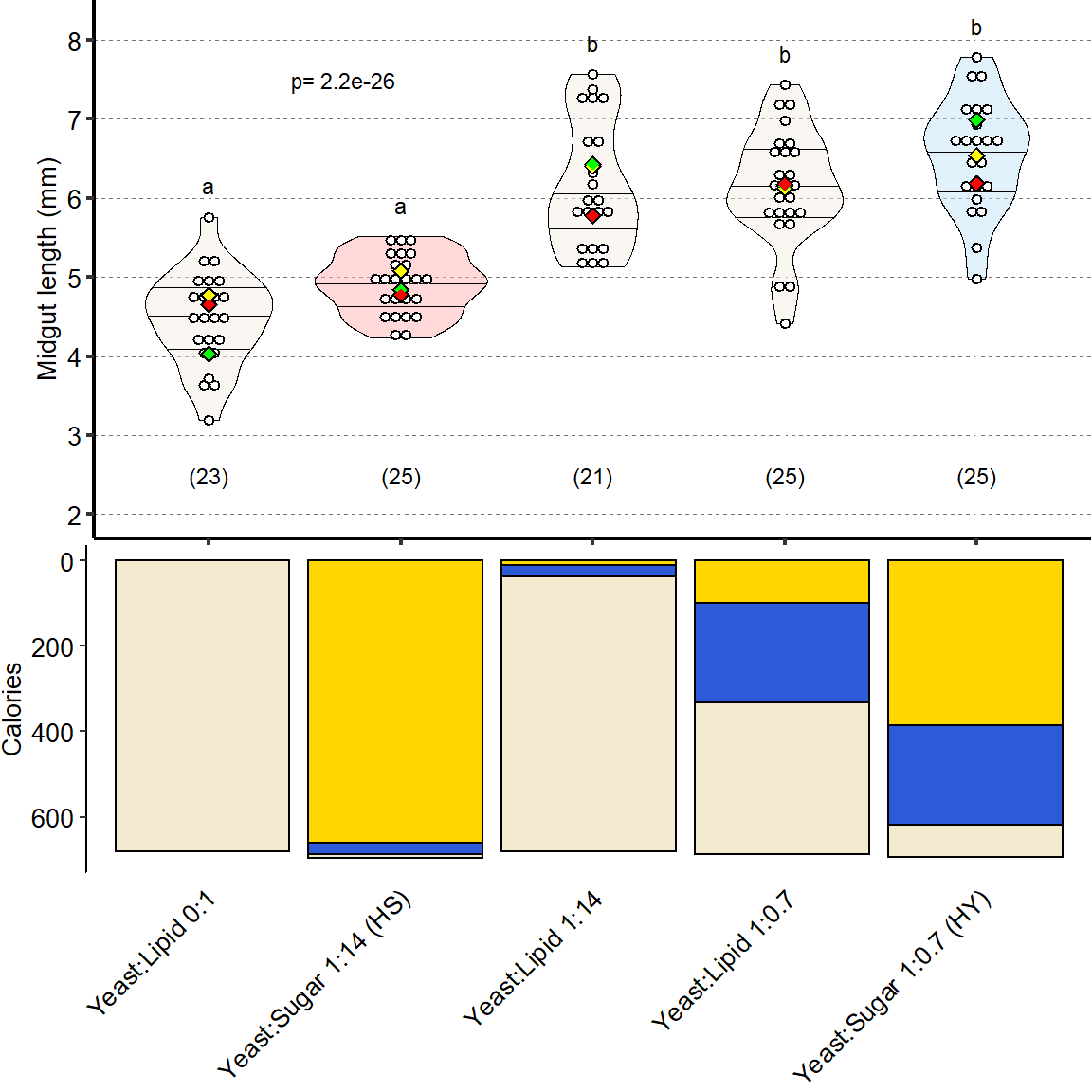
2.1.7 Figure 2G
Antagonism by sugar of yeast-induced growth is not specific to sucrose. Statistical comparisons were performed with HS vs HY for each sugar.
tab_sugars =
  d[["2G"]]%>%
  mutate(Total_Length_mm =Total.L/1000)%>%
  mutate_if(is.character,as.factor)%>%
  mutate_if(is.integer,as.factor)%>%
  dplyr::rename(Day_of_Treatment=Day)

tab_sugars$Sugar = factor(c("Sucrose","Fructose","Glucose","Maltose"), levels = c("Sucrose", "Glucose", "Fructose", "Maltose"))

Sample_size=
  tab_sugars%>%
  group_by(Diet,Sugar)%>%
  summarise(Sample_size=n())

###Stats
# Sucrose:
mod.gen = fitme(log(Total_Length_mm) ~  Diet + (1 | Repeat), data = subset(tab_sugars,Sugar=="Sucrose"))
shapiro.test(residuals(mod.gen))
    Shapiro-Wilk normality test

data:  residuals(mod.gen)
W = 0.98398, p-value = 0.9186bptest(log(Total_Length_mm) ~ Diet + (1 / Repeat), data = subset(tab_sugars,Sugar=="Sucrose"))
    studentized Breusch-Pagan test

data:  log(Total_Length_mm) ~ Diet + (1/Repeat)
BP = 0.52599, df = 1, p-value = 0.4683
mod.gen1 = fitme(log(Total_Length_mm) ~ 1 + (1 | Repeat), data = subset(tab_sugars,Sugar=="Sucrose"))
test = anova(mod.gen, mod.gen1)
Chi2_LRT_growth = 2*(mod.gen$APHLs[["p_v"]]-mod.gen1$APHLs[["p_v"]])
tab_stat = data.frame(Variable = as.character(paste("HS vs HY sucrose")),
Rep = nlevels(tab_lipids$Repeat),
chi2_LR = round(as.numeric(test$basicLRT$chi2_LR), digits = 2),
intercept = format(mod.gen$fixef[1],digits=3),
estimate = format(mod.gen$fixef[2],digits=3),
df = as.numeric(test$basicLRT$df),
Pvalue = as.numeric(format(pchisq(Chi2_LRT_growth,df=1,lower.tail = F),digits=2)))
tab_stat_sucrose =tab_stat
# Glucose:
mod.gen = fitme(log(Total_Length_mm) ~ Diet + (1 | Repeat), data = subset(tab_sugars,Sugar=="Glucose"))
shapiro.test(residuals(mod.gen))
    Shapiro-Wilk normality test

data:  residuals(mod.gen)
W = 0.94939, p-value = 0.1628bptest(log(Total_Length_mm) ~ Diet + (1 / Repeat), data = subset(tab_sugars,Sugar=="Glucose"))
    studentized Breusch-Pagan test

data:  log(Total_Length_mm) ~ Diet + (1/Repeat)
BP = 0.92415, df = 1, p-value = 0.3364
mod.gen1 = fitme(log(Total_Length_mm) ~ 1 + (1 | Repeat), data = subset(tab_sugars,Sugar=="Glucose"))
test = anova(mod.gen, mod.gen1)
Chi2_LRT_growth = 2*(mod.gen$APHLs[["p_v"]]-mod.gen1$APHLs[["p_v"]])
tab_stat = data.frame(Variable = as.character(paste("HS vs HY glucose")),
Rep = nlevels(tab_lipids$Repeat),
chi2_LR = round(as.numeric(test$basicLRT$chi2_LR), digits = 2),
intercept = format(mod.gen$fixef[1],digits=3),
estimate = format(mod.gen$fixef[2],digits=3),
df = as.numeric(test$basicLRT$df),
Pvalue = as.numeric(format(pchisq(Chi2_LRT_growth,df=1,lower.tail = F),digits=2)))
tab_stat_Glucose=tab_stat
# Fructose:
mod.gen = fitme(log(Total_Length_mm) ~ Diet + (1 | Repeat), data = subset(tab_sugars,Sugar=="Fructose"))
shapiro.test(residuals(mod.gen))
    Shapiro-Wilk normality test

data:  residuals(mod.gen)
W = 0.96101, p-value = 0.3101bptest(log(Total_Length_mm) ~ Diet + (1 / Repeat), data = subset(tab_sugars,Sugar=="Fructose"))
    studentized Breusch-Pagan test

data:  log(Total_Length_mm) ~ Diet + (1/Repeat)
BP = 0.80035, df = 1, p-value = 0.371
mod.gen1 = fitme(log(Total_Length_mm) ~ 1 + (1 | Repeat), data = subset(tab_sugars,Sugar=="Fructose"))
test = anova(mod.gen, mod.gen1)
Chi2_LRT_growth = 2*(mod.gen$APHLs[["p_v"]]-mod.gen1$APHLs[["p_v"]])
tab_stat = data.frame(Variable = as.character(paste("HS vs HY fructose")),
Rep = nlevels(tab_lipids$Repeat),
chi2_LR = round(as.numeric(test$basicLRT$chi2_LR), digits = 2),
intercept = format(mod.gen$fixef[1],digits=3),
estimate = format(mod.gen$fixef[2],digits=3),
df = as.numeric(test$basicLRT$df),
Pvalue = as.numeric(format(pchisq(Chi2_LRT_growth,df=1,lower.tail = F),digits=2)))
tab_stat_Fructose = tab_stat
# Maltose:
mod.gen = fitme(log(Total_Length_mm) ~ Diet + (1 | Repeat), data = subset(tab_sugars,Sugar=="Maltose"))
shapiro.test(residuals(mod.gen))
    Shapiro-Wilk normality test

data:  residuals(mod.gen)
W = 0.94774, p-value = 0.1352bptest(log(Total_Length_mm) ~ Diet + (1 / Repeat), data = subset(tab_sugars,Sugar=="Maltose"))
    studentized Breusch-Pagan test

data:  log(Total_Length_mm) ~ Diet + (1/Repeat)
BP = 0.080366, df = 1, p-value = 0.7768
mod.gen1 = fitme(log(Total_Length_mm) ~ 1 + (1 | Repeat), data = subset(tab_sugars,Sugar=="Maltose"))
test = anova(mod.gen, mod.gen1)
Chi2_LRT_growth = 2*(mod.gen$APHLs[["p_v"]]-mod.gen1$APHLs[["p_v"]])
tab_stat = data.frame(Variable = as.character(paste("HS vs HY maltose")),
Rep = nlevels(tab_lipids$Repeat),
chi2_LR = round(as.numeric(test$basicLRT$chi2_LR), digits = 2),
intercept = format(mod.gen$fixef[1],digits=3),
estimate = format(mod.gen$fixef[2],digits=3),
df = as.numeric(test$basicLRT$df),
Pvalue = as.numeric(format(pchisq(Chi2_LRT_growth,df=1,lower.tail = F),digits=2)))
tab_stat_Maltose= tab_stat
tab_stat = rbind(tab_stat_sucrose,tab_stat_Glucose,tab_stat_Fructose,tab_stat_Maltose)
tab_stat$sig = ifelse(tab_stat$Pvalue < 0.05 & tab_stat$Pvalue > 0.01, "*",
ifelse(tab_stat$Pvalue < 0.01 & tab_stat$Pvalue > 0.001, "**",
ifelse(tab_stat$Pvalue < 0.001, "***", "")))
tab_stat$Sugar = c("Sucrose","Glucose","Fructose","Maltose")
tab_stat$Sugar =as.factor(tab_stat$Sugar)
tab_stat%>%
kable(col.names = c("Comparison", "Replicates", "Chi2","Intercept","Estimate","df" ,"p-value","Signif.","Sugar"),row.names = FALSE) %>% add_header_above(c("log(Total_Length_mm) ~ Diet + (1 | Repeat)" = 9))%>%
kable_styling(bootstrap_options = c("striped", "hover", "condensed"), full_width = F)| Comparison | Replicates | Chi2 | Intercept | Estimate | df | p-value | Signif. | Sugar |
|---|---|---|---|---|---|---|---|---|
| HS vs HY sucrose | 3 | 42.83 | 1.56 | 0.333 | 1 | 0.0e+00 | *** | Sucrose |
| HS vs HY glucose | 3 | 16.16 | 1.6 | 0.218 | 1 | 5.8e-05 | *** | Glucose |
| HS vs HY fructose | 3 | 39.14 | 1.53 | 0.32 | 1 | 0.0e+00 | *** | Fructose |
| HS vs HY maltose | 3 | 20.75 | 1.54 | 0.244 | 1 | 5.2e-06 | *** | Maltose |
Limits = c("HS","HY")
Labels= c("HS","HY")

z = max(tab_sugars$Total_Length_mm, na.rm = TRUE)

Plot_Fig2G=
  ggplot(tab_sugars, aes(x = Diet, y = Total_Length_mm))+
  geom_violin(aes(fill = Diet), draw_quantiles = c(0.25, 0.5, 0.75), colour = "black", size = 0.2,adjust = 0.8) +
  geom_dotplot(colour = "black", fill = "white", binaxis = "y", stackdir = "center", binwidth = z / 60) +
  geom_text(data = Sample_size, mapping = aes(x = Diet, y = 2.5, label = paste("(",Sample_size,")",sep="")),size=3)+
  geom_signif(data = tab_stat,aes(xmin = 1, xmax = 2, annotations = formatC(paste("p=",Pvalue), digits = 2), y_position = 8.5), textsize = 3, vjust = -0.2, manual = TRUE)+
  facet_grid(.~Sugar)+
  scale_fill_manual(limits=Limits,
                    values=palette_diet_2)+
  scale_x_discrete("",
                   limits=Limits,
                   labels=Labels)+
  scale_y_continuous("Midgut length (mm)",
                     limits=c(2,9),
                     breaks=seq(2,8,by=1))+
   stat_summary(fun = mean, geom = "point", size = 3, shape = 18, colour = "black", aes(group = Repeat)) +
                     stat_summary(fun = mean, geom = "point", size = 2, shape = 18, aes(group = Repeat, colour = Repeat)) +
                     scale_color_manual(values = palette_mean) +
  theme(panel.background = element_blank(),
        panel.grid.major.y = element_line(colour = grey(0.45), linetype = "dashed", size = 0.2),
        axis.title.x = element_blank(),
        axis.title.y = element_text(size=Smallfont,colour="black"),
        axis.line.x = element_line(colour="black",size=0.75),
        axis.line.y = element_line(colour="black",size=0.75),
        axis.ticks.x = element_line(size = 0.75),
        axis.ticks.y = element_line(size = 0.75),
        axis.text.x = element_text(size=Smallfont,colour="black"),
        axis.text.y = element_text(size=Smallfont,colour="black"),
        plot.margin = unit(c(0,0,0,0.5), "cm"),
        legend.direction = "vertical",
        legend.box = "horizontal",
        legend.position = "none",
        legend.key.height = unit(0.4, "cm"),
        legend.key.width= unit(0.6, "cm"),
        legend.title = element_text(face="italic",size=Smallfont),
        legend.key = element_rect(colour = 'white', fill = "white", linetype='dashed'),
        legend.text = element_text(size=SuperSmallfont),
        legend.background = element_rect(fill=NA),
        strip.text.x = element_text(size = Smallfont, colour = "black", margin = margin(t = 2, r = 0, b = 2, l = 0)),
        strip.text.y = element_text(size = Smallfont, colour = "black", margin = margin(t = 2, r = 0, b = 2, l = 0)),
        strip.background = element_rect(fill=NA, colour="black"),
        strip.placement="outside")

Plot_Fig2G
##Export Figure 2
2.2 Figure 2 - figure supplement 1
2.2.1 Figure 2S1A
Set of diets utilized for the nutritional geometry experiment. Numbers on dots denote sample sizes for figure 2A (pool of three independent biological replicates). We utilized 28 different diets, varying either caloric content or the yeast to sucrose ratio. The complete list of recipes can be found in Table 1. Complete numbers can be found in manuscript figure
tab_nutri_geo_design =
  d[["2 - S1A"]]%>%
  dplyr::rename(Yeast.in.Diet=Yeast,
         Sucrose.in.Diet=Sugar)

tab_raw_2A =
  d[["2A"]]%>%
  mutate_if(is.character,as.factor)%>%
  mutate_if(is.integer,as.factor)%>%
  mutate(Conc = paste(round(Sucrose.in.Diet,digits=2),"x",round(Yeast.in.Diet,digits=2),sep=""))%>%
  group_by(Yeast.in.Diet,Sucrose.in.Diet)%>%
  summarise(Sample_size=n())

tab_nutri_geo_design = left_join(tab_nutri_geo_design,tab_raw_2A)

Plot_Fig2S1A=
  ggplot(tab_nutri_geo_design, aes(x = Sucrose.in.Diet, y = Yeast.in.Diet,label=Sample_size))+
  geom_point(aes(size=Calories), colour = "black") +
  scale_x_continuous("Sucrose in diet (g/L)",
                     limits=c(-5,300),
                     breaks=seq(0,300,by=100))+
  scale_y_continuous("Yeast in diet (g/L)",
                     limits=c(-5,300),
                     breaks=seq(0,300,by=100))+
  geom_text(data=subset(tab_nutri_geo_design,Yeast.in.Diet>=30 | Sucrose.in.Diet>=30),color="white",size=3)+
  scale_size_continuous(range = c(1,13)) +
  theme(panel.background = element_blank(),
        panel.grid.major = element_line(colour = "black",linetype=3),
        axis.title.x = element_text(size=Smallfont,colour="black"),
        axis.title.y = element_text(size=Smallfont,colour="black"),
        axis.line.x = element_line(colour="black",size=0.75),
        axis.line.y = element_line(colour="black",size=0.75),
        axis.ticks.x = element_line(size = 0.75),
        axis.ticks.y = element_line(size = 0.75),
        axis.text.x = element_text(size=Smallfont,colour="black"),
        axis.text.y = element_text(size=Smallfont,colour="black"),
        plot.margin = unit(c(0,0,0,0.5), "cm"),
        legend.direction = "horizontal",
        legend.box = "horizontal",
        legend.position = "top",
        legend.key.height = unit(0.4, "cm"),
        legend.key.width= unit(0.6, "cm"),
        legend.title = element_text(face="italic",size=Smallfont),
        legend.key = element_rect(colour = 'white', fill = "white", linetype='dashed'),
        legend.text = element_text(size=SuperSmallfont),
        legend.background = element_rect(fill=NA),
        strip.text.x = element_text(size =Smallfont, colour = "black",face="italic"),
        strip.text.y = element_text(size =Smallfont, colour = "black",face="italic"),
        strip.background = element_rect(fill=NA, colour="black"),
        strip.placement="outside")+
  guides(size=guide_legend(ncol=4))

Plot_Fig2S1A
HS and HY diet compared to standard diets used for Drosophila
2.2.2 Figure 2S1B
FD&C1 blue transit assay (feeding assay) showing amount of food defecated, and by inference ingested, in the nutritional geometry experiment. The scale maps color to units. The graph indicates compensatory feeding at lower nutrient densities, especially low yeast. These data were used to calculate the total amount of yeast and sucrose ingested on each diet in Figure 2-supplemental figure 1C.
tab_geom_fecal =
  d[["2 - S1B"]]

jpeg(filename = "F:/Dropbox/Github/Bonfini_eLife_2021/data/Plot_Fig2-S1B.jpeg",
     res = 600,
     width = 5, height = 4, units = 'in' )
par(cex=1, mar = c(4, 4, 1, 3))
with(tab_geom_fecal, geomPlotta(x = Sucrose.in.Diet, y = Yeast.in.Diet, z = (Absorbance*10), alf = 1, xlim = c(-10, 300), ylim = c(-10, 300), xlab = "Sucrose in diet (g/L)", ylab = "Yeast in diet (g/L)", frame.plot= FALSE, cex.lab=1, cex.axis =1, las=1, labcex=1, asp=1))
img2S1B = readImage("F:/Dropbox/Github/Bonfini_eLife_2021/data/Plot_Fig2-S1B.jpeg")
gob_imageFig2S1B = rasterGrob(img2S1B)
grid.draw(gob_imageFig2S1B)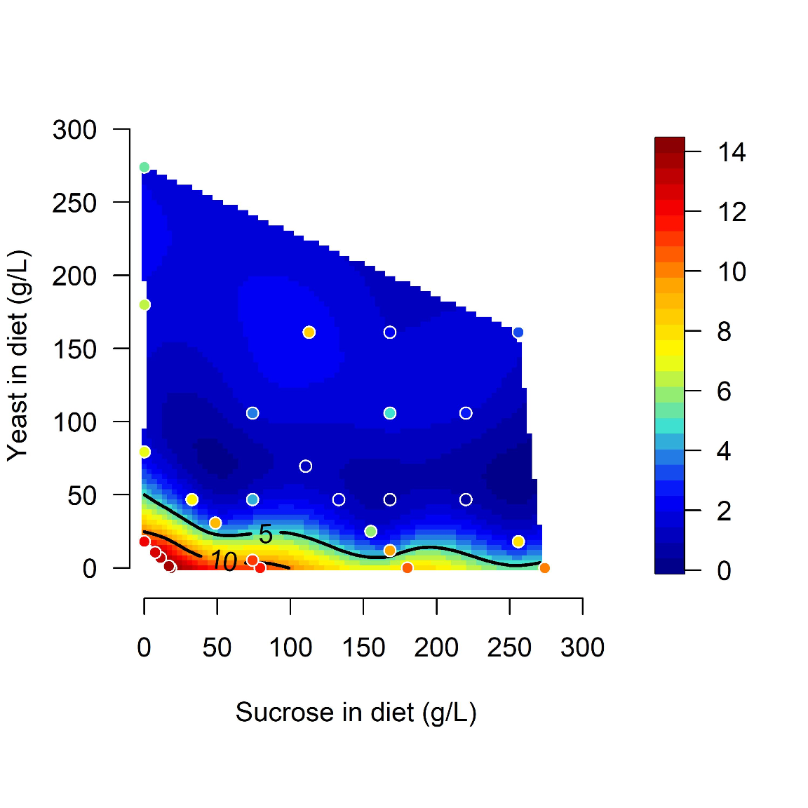
2.2.3 Figure 2S1C
Yeast and sucrose have mutually antagonistic impacts on midgut length. Plots show midgut length as a function of sucrose or yeast ingested (g/L x Absorbance from Figure 2-supplemental figure 1B), or their ratio multiplied by ingestion per diet.
tab_nutri_geo =
  d[["2A"]]%>%
    mutate(Total.Lmm = Total.L / 1000)

tab_nutri_geo2 <- tab_nutri_geo %>%
    group_by(concatenate) %>%
    summarize(Calories.ingested = mean(Calories.ingested),
              Midgut.length = mean(Total.Lmm),
              Yeast.ingested = mean(Yeast.ingested),
              Sucrose.ingested = mean(Sucrose.ingested))

graph <- ggplot(tab_nutri_geo2, aes(x=Sucrose.ingested, y=Yeast.ingested))

Plot_Fig2S1C=
  graph + geom_point(aes(size=Calories.ingested, fill=Midgut.length), stroke=1.5, shape=21,  color="black") +
  scale_size(range = c(1,5)) +
  scale_fill_viridis_c() +
  theme(plot.title= element_text(hjust = 0.5))+
  scale_x_continuous("Sucrose ingested (g/L x Absorbance)",
                     limits=c(-5,160),
                     breaks=seq(0,160,by=25))+
  scale_y_continuous("Yeast ingested (g/L x Absorbance)",
                     limits=c(-5,50),
                     breaks=seq(0,50,by=10))+
  scale_size_continuous(range = c(1,10)) +
  theme(panel.background = element_blank(),
        panel.grid.major = element_line(colour = "black",linetype=3),
        axis.title.x = element_text(size=Smallfont,colour="black"),
        axis.title.y = element_text(size=Smallfont,colour="black"),
        axis.line.x = element_line(colour="black",size=0.75),
        axis.line.y = element_line(colour="black",size=0.75),
        axis.ticks.x = element_line(size = 0.75),
        axis.ticks.y = element_line(size = 0.75),
        axis.text.x = element_text(size=Smallfont,colour="black"),
        axis.text.y = element_text(size=Smallfont,colour="black"),
        plot.margin = unit(c(0,0,0,0.5), "cm"),
        legend.direction = "horizontal",
        legend.box = "vertical",
        legend.position = c(0.79,0.79),
        legend.key.height = unit(0.3, "cm"),
        legend.key.width= unit(0.4, "cm"),
        legend.title = element_text(face="italic",size=Smallfont),
        legend.key = element_rect(colour = 'white', fill = "white", linetype='dashed'),
        legend.text = element_text(size=SuperSmallfont),
        strip.text.x = element_text(size =Smallfont, colour = "black",face="italic"),
        strip.text.y = element_text(size =Smallfont, colour = "black",face="italic"),
        strip.background = element_rect(fill=NA, colour="black"),
        strip.placement="outside")+
  labs(fill = "Midgut length (mm)", size = "Calories ingested")

Plot_Fig2S1C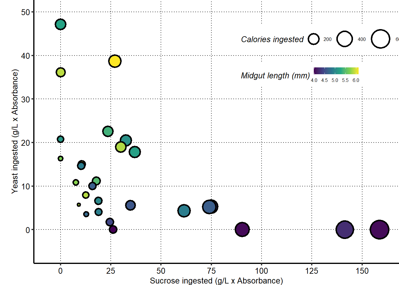
##Export Figure 2S1
2.3 Figure 2 - figure supplement 2
2.3.1 Figure 2S2A
Food texture does not explain the differential effects of HS and HY diets on midgut length. Addition of inulin (inu), pectin (pect), cellulose (cell), and all previous fibers mixed (AF) or pectin + cellulose (PC) to HS does not increase midgut length. Addition of fibers to HY (HY + AF) and HY + pectin + cellulose (HY + PC2) does not affect midgut length.
tab_fiber =
  d[["2 - S2A"]]%>%
  mutate_if(is.character,as.factor)%>%
  mutate_if(is.integer,as.factor)%>%
  mutate(Total_Length_mm = Total.L/1000)%>%
  dplyr::rename(Diet=Food)

tab_fiber$Diet = factor(tab_fiber$Diet, levels = c("HS", "HS + Inu", "HS + Pect", "HS + Pect2", "HS + Cell", "HS + Cell2", "HS + AF", "HS + PC2", "HY + AF", "HY + PC2", "HY"))

Sample_size=
  tab_fiber%>%
  group_by(Diet)%>%
  summarise(Sample_size=n())

###Stats

mod.gen = fitme(log(Total_Length_mm) ~  Diet + (1 | Repeat), data = tab_fiber)
shapiro.test(residuals(mod.gen))
    Shapiro-Wilk normality test

data:  residuals(mod.gen)
W = 0.9942, p-value = 0.4463bptest(log(Total_Length_mm) ~ Diet + (1 / Repeat), data = tab_fiber)
    studentized Breusch-Pagan test

data:  log(Total_Length_mm) ~ Diet + (1/Repeat)
BP = 7.5012, df = 10, p-value = 0.6774
mod.gen1 = fitme(log(Total_Length_mm) ~ 1 + (1 | Repeat), data = tab_fiber)
test = anova(mod.gen, mod.gen1)
Chi2_LRT_growth = 2*(mod.gen$APHLs[["p_v"]]-mod.gen1$APHLs[["p_v"]])
#Now we make a tab with the results
tab_stat = data.frame(Variable = as.character(paste("Any difference")),
Rep = nlevels(tab_fiber$Repeat),
chi2_LR = round(as.numeric(test$basicLRT$chi2_LR), digits = 2),
intercept = format(mod.gen$fixef[1],digits=3),
estimate = format(mod.gen$fixef[2],digits=3),
df = as.numeric(test$basicLRT$df),
Pvalue = as.numeric(format(pchisq(Chi2_LRT_growth,df=1,lower.tail = F),digits=2)))
tab_stat$sig = ifelse(tab_stat$Pvalue < 0.05 & tab_stat$Pvalue > 0.01, "*",
ifelse(tab_stat$Pvalue < 0.01 & tab_stat$Pvalue > 0.001, "**",
ifelse(tab_stat$Pvalue < 0.001, "***", "")))
tab_stat%>%
kable(col.names = c("Comparison", "Replicates", "Chi2","Intercept","Estimate","df" ,"p-value","Signif."),row.names = FALSE) %>% add_header_above(c("log(Total_Length_mm) ~ Diet + (1 | Repeat)" = 8))%>%
kable_styling(bootstrap_options = c("striped", "hover", "condensed"), full_width = F)| Comparison | Replicates | Chi2 | Intercept | Estimate | df | p-value | Signif. |
|---|---|---|---|---|---|---|---|
| Any difference | 3 | 122.76 | 1.55 | -0.0361 | 10 | 0 | *** |
mod.gen = lmer(Total_Length_mm ~  Diet + (1 | Repeat), data = tab_fiber)
multcomp = glht(mod.gen, linfct=mcp(Diet="Tukey"))

tmp = cld(multcomp)

letter_position = aggregate(data=subset(tab_fiber,!is.na(Total_Length_mm)),Total_Length_mm ~ Diet, max)

tab_letter =  as.data.frame(tmp$mcletters$Letters)
tab_letter$Diet=rownames(tab_letter)
colnames(tab_letter)[1] = "Letter"
tab_letter = left_join(tab_letter,letter_position)

### Plot

Limits= c("HS", "HS + Inu", "HS + Pect", "HS + Pect2", "HS + Cell", "HS + Cell2", "HS + AF", "HS + PC2", "HY + AF", "HY + PC2", "HY")

cbbPalette = c("#FFB4B4", "#f6efe5", "#f6efe5", "#f6efe5", "#f6efe5", "#f6efe5", "#f6efe5","#f6efe5", "#f6efe5", "#f6efe5", "#C3E6FC")
z = max(tab_fiber$Total_Length_mm, na.rm = TRUE)

Plot_Fig2S2A=
  ggplot(tab_fiber, aes(x = Diet, y = Total_Length_mm))+
  geom_violin(aes(fill = Diet), draw_quantiles = c(0.25, 0.5, 0.75), colour = "black", size = 0.2,adjust = 0.8) +
  geom_dotplot( colour = "black", fill = "white", binaxis = "y", stackdir = "center", binwidth = z/60) +
  geom_text(data = Sample_size, mapping = aes(x = Diet, y = 2.5, label = paste("(",Sample_size,")",sep="")),size=3)+
  geom_text(data = tab_letter, mapping = aes(x = Diet, y = Total_Length_mm+0.4, label = Letter),size=3)+
  geom_text(data = tab_stat, mapping = aes(x = 1.5, y = 7.5, label = paste("p=",format(Pvalue,digits=2))),size=3)+
  scale_fill_manual(limits=Limits,
                    values=cbbPalette)+
  scale_x_discrete("",
                   limits=Limits)+
  scale_y_continuous("Midgut length (mm)",
                     limits=c(2,8),
                     breaks=seq(2,8,by=1))+
  stat_summary(fun = mean, geom = "point", size = 3, shape = 18, colour = "black", aes(group = Repeat)) +
  stat_summary(fun = mean, geom = "point", size = 2, shape = 18, aes(group = Repeat, colour = Repeat)) +
  scale_color_manual(values = palette_mean) +
  theme(panel.background = element_blank(),
        panel.grid.major.y = element_line(colour = grey(0.45), linetype = "dashed", size = 0.2),
        axis.title.x = element_blank(),
        axis.title.y = element_text(size=Smallfont,colour="black"),
        axis.line.x = element_line(colour="black",size=0.75),
        axis.line.y = element_line(colour="black",size=0.75),
        axis.ticks.x = element_line(size = 0.75),
        axis.ticks.y = element_line(size = 0.75),
        axis.text.x = element_text(size=Smallfont,colour="black",angle=45,hjust=1),
        axis.text.y = element_text(size=Smallfont,colour="black"),
        plot.margin = unit(c(0,0,0,0.5), "cm"),
        legend.direction = "vertical",
        legend.box = "horizontal",
        legend.position = "none",
        legend.key.height = unit(0.4, "cm"),
        legend.key.width= unit(0.6, "cm"),
        legend.title = element_text(face="italic",size=Smallfont),
        legend.key = element_rect(colour = 'white', fill = "white", linetype='dashed'),
        legend.text = element_text(size=SuperSmallfont),
        legend.background = element_rect(fill=NA))

Plot_Fig2S2A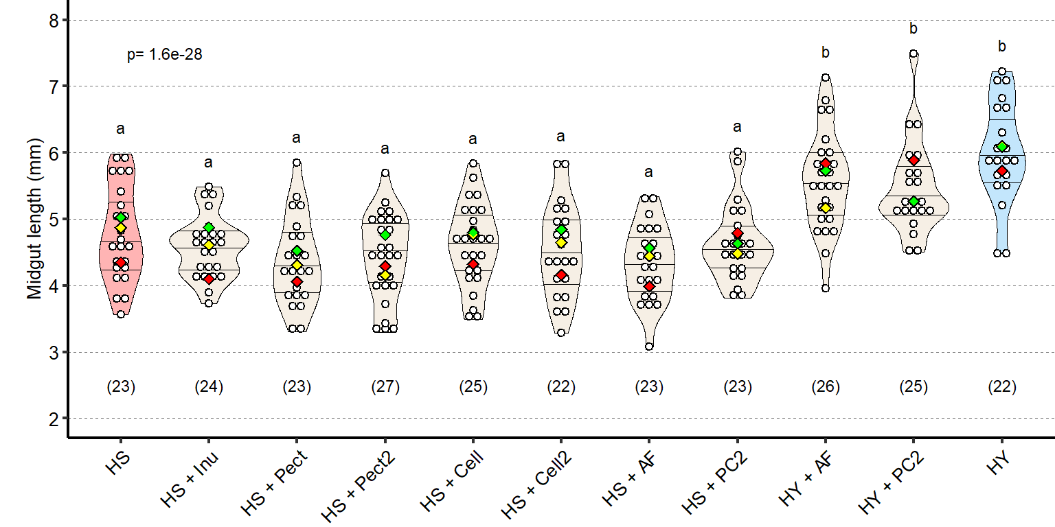
2.3.2 Figure 2S2B
Changes in food texture due to variation in agar concentration can affect midgut length but do not explain the effect of the diet treatment. Changes in agar concentration do not change midgut length on HS. Either increasing or decreasing agar concentration reduces midgut length on HY.
tab_agar =
  d[["2 - S2B"]]%>%
  mutate_if(is.character,as.factor)%>%
  mutate_if(is.integer,as.factor)%>%
  mutate(Total_Length_mm = Total.L/1000)%>%
  dplyr::rename(Diet=Food)

levels(tab_agar$Diet)[levels(tab_agar$Diet)=="HS"] ="HS (original, 1.5%)"
levels(tab_agar$Diet)[levels(tab_agar$Diet)=="HY"] ="HY (original, 1.5%)"

Sample_size=
  tab_agar%>%
  group_by(Diet)%>%
  summarise(Sample_size=n())

###Stats

mod.gen = fitme(log(Total_Length_mm) ~  Diet + (1 | Repeat), data = tab_agar)
shapiro.test(residuals(mod.gen))
    Shapiro-Wilk normality test

data:  residuals(mod.gen)
W = 0.99568, p-value = 0.4148bptest(log(Total_Length_mm) ~ Diet + (1 / Repeat), data = tab_agar)
    studentized Breusch-Pagan test

data:  log(Total_Length_mm) ~ Diet + (1/Repeat)
BP = 5.8743, df = 7, p-value = 0.5545
mod.gen1 = fitme(log(Total_Length_mm) ~ 1 + (1 | Repeat), data = tab_agar)
test = anova(mod.gen, mod.gen1)
Chi2_LRT_growth = 2*(mod.gen$APHLs[["p_v"]]-mod.gen1$APHLs[["p_v"]])
#Now we make a tab with the results
tab_stat = data.frame(Variable = as.character(paste("Any difference")),
Rep = nlevels(tab_agar$Repeat),
chi2_LR = round(as.numeric(test$basicLRT$chi2_LR), digits = 2),
intercept = format(mod.gen$fixef[1],digits=3),
estimate = format(mod.gen$fixef[2],digits=3),
df = as.numeric(test$basicLRT$df),
Pvalue = as.numeric(format(pchisq(Chi2_LRT_growth,df=1,lower.tail = F),digits=2)))
tab_stat$sig = ifelse(tab_stat$Pvalue < 0.05 & tab_stat$Pvalue > 0.01, "*",
ifelse(tab_stat$Pvalue < 0.01 & tab_stat$Pvalue > 0.001, "**",
ifelse(tab_stat$Pvalue < 0.001, "***", "")))
tab_stat%>%
kable(col.names = c("Comparison", "Replicates", "Chi2","Intercept","Estimate","df" ,"p-value","Signif."),row.names = FALSE) %>% add_header_above(c("log(Total_Length_mm) ~ Diet + (1 | Repeat)" = 8))%>%
kable_styling(bootstrap_options = c("striped", "hover", "condensed"), full_width = F)| Comparison | Replicates | Chi2 | Intercept | Estimate | df | p-value | Signif. |
|---|---|---|---|---|---|---|---|
| Any difference | 6 | 201.35 | 1.49 | -5.9e-05 | 7 | 0 | *** |
mod.gen = lmer(Total_Length_mm ~  Diet + (1 | Repeat), data = tab_agar)
multcomp = glht(mod.gen, linfct=mcp(Diet="Tukey"))

tmp = cld(multcomp)

letter_position = aggregate(data=subset(tab_agar,!is.na(Total_Length_mm)),Total_Length_mm ~ Diet, max)

tab_letter =  as.data.frame(tmp$mcletters$Letters)
tab_letter$Diet=rownames(tab_letter)
colnames(tab_letter)[1] = "Letter"
tab_letter = left_join(tab_letter,letter_position)

### Plot

Limits= c("HS Agar 0.5%", "HS Agar 1%", "HS (original, 1.5%)", "HS Agar 3%", "HY Agar 0.5%", "HY Agar 1%", "HY (original, 1.5%)", "HY Agar 3%")

cbbPalette = c("#FFB4B4", "#FFB4B4", "#FFB4B4", "#FFB4B4", "#C3E6FC", "#C3E6FC", "#C3E6FC", "#C3E6FC")
z = max(tab_agar$Total_Length_mm, na.rm = TRUE)

Plot_Fig2S2B=
  ggplot(tab_agar, aes(x = Diet, y = Total_Length_mm))+
  geom_violin(aes(fill = Diet), draw_quantiles = c(0.25, 0.5, 0.75), colour = "black", size = 0.2,adjust = 0.8) +
  geom_dotplot( colour = "black", fill = "white", binaxis = "y", stackdir = "center", binwidth = z/60) +
  geom_text(data = Sample_size, mapping = aes(x = Diet, y = 2.5, label = paste("(",Sample_size,")",sep="")),size=3)+
  geom_text(data = tab_letter, mapping = aes(x = Diet, y = Total_Length_mm+0.4, label = Letter),size=3)+
  geom_text(data = tab_stat, mapping = aes(x = 1.5, y = 7.5, label = paste("p=",Pvalue)),size=3)+
  scale_fill_manual(limits=Limits,
                    values=cbbPalette)+
  scale_x_discrete("",
                   limits=Limits)+
  scale_y_continuous("Midgut length (mm)",
                     limits=c(2,8),
                     breaks=seq(2,8,by=1))+
  stat_summary(fun = mean, geom = "point", size = 3, shape = 18, colour = "black", aes(group = Repeat)) +
  stat_summary(fun = mean, geom = "point", size = 2, shape = 18, aes(group = Repeat, colour = Repeat)) +
  scale_color_manual(values = palette_mean) +
  theme(panel.background = element_blank(),
        panel.grid.major.y = element_line(colour = grey(0.45), linetype = "dashed", size = 0.2),
        axis.title.x = element_blank(),
        axis.title.y = element_text(size=Smallfont,colour="black"),
        axis.line.x = element_line(colour="black",size=0.75),
        axis.line.y = element_line(colour="black",size=0.75),
        axis.ticks.x = element_line(size = 0.75),
        axis.ticks.y = element_line(size = 0.75),
        axis.text.x = element_text(size=Smallfont,colour="black",angle=34,hjust=1),
        axis.text.y = element_text(size=Smallfont,colour="black"),
        plot.margin = unit(c(0,0,0,0.5), "cm"),
        legend.direction = "vertical",
        legend.box = "horizontal",
        legend.position = "none",
        legend.key.height = unit(0.4, "cm"),
        legend.key.width= unit(0.6, "cm"),
        legend.title = element_text(face="italic",size=Smallfont),
        legend.key = element_rect(colour = 'white', fill = "white", linetype='dashed'),
        legend.text = element_text(size=SuperSmallfont),
        legend.background = element_rect(fill=NA))

Plot_Fig2S2B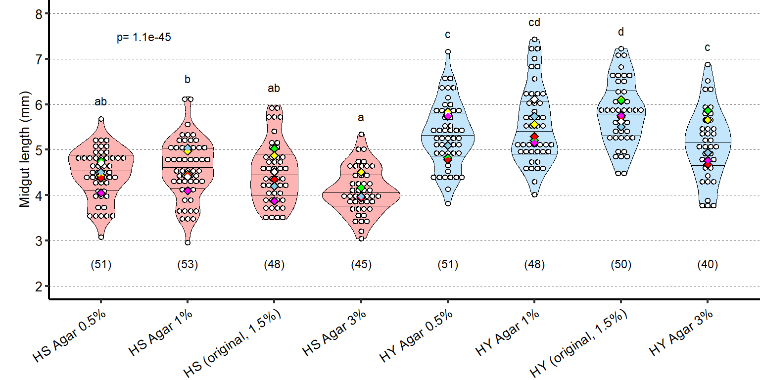
2.3.3 Figure 2S2C
Sorbitol, a nutritious but not palatable sugar, has increased size on HY compared to HS, while Arabinose, a palatable but not nutritious sugar, results in death of flies before reaching dissection day on HS, and decreased size of midguts on HY diet. Statistical analysis is HS vs HY for each sugar.
tab_xtrsugars_rev =
  d[["2S2C"]]%>%
  mutate(Total_Length_mm =Total.L/1000)%>%
  mutate_if(is.character,as.factor)%>%
  mutate_if(is.integer,as.factor)%>%
  dplyr::rename(Day_of_Treatment=Day)%>%
  mutate(Sugar=fct_relevel(Sugar,"Sucrose","Sorbitol", "Arabinose"))

#tab_xtrsugars_rev$Sugar = factor(c("Sucrose","Sorbitol","Arabinose"), levels = c("Sucrose", "Sorbitol", "Arabinose"))

Sample_size=
  tab_xtrsugars_rev%>%
  group_by(Diet,Sugar)%>%
  summarise(Sample_size=n())

###Stats
# Sucrose:
mod.gen = fitme((Total_Length_mm) ~  Diet + (1 | Repeat), data = subset(tab_xtrsugars_rev,Sugar=="Sucrose"))
shapiro.test(residuals(mod.gen))
    Shapiro-Wilk normality test

data:  residuals(mod.gen)
W = 0.96327, p-value = 0.07213bptest((Total_Length_mm) ~ Diet + (1 / Repeat), data = subset(tab_xtrsugars_rev,Sugar=="Sucrose"))
    studentized Breusch-Pagan test

data:  (Total_Length_mm) ~ Diet + (1/Repeat)
BP = 0.77017, df = 1, p-value = 0.3802
mod.gen1 = fitme((Total_Length_mm) ~ 1 + (1 | Repeat), data = subset(tab_xtrsugars_rev,Sugar=="Sucrose"))
test = anova(mod.gen, mod.gen1)
Chi2_LRT_growth = 2*(mod.gen$APHLs[["p_v"]]-mod.gen1$APHLs[["p_v"]])
tab_stat = data.frame(Variable = as.character(paste("HS vs HY Sucrose")),
Rep = nlevels(tab_lipids$Repeat),
chi2_LR = round(as.numeric(test$basicLRT$chi2_LR), digits = 2),
intercept = format(mod.gen$fixef[1],digits=3),
estimate = format(mod.gen$fixef[2],digits=3),
df = as.numeric(test$basicLRT$df),
Pvalue = as.numeric(format(pchisq(Chi2_LRT_growth,df=1,lower.tail = F),digits=2)))
tab_stat_sucrose =tab_stat
# Sorbitol:
mod.gen = fitme((Total_Length_mm) ~ Diet + (1 | Repeat), data = subset(tab_xtrsugars_rev,Sugar=="Sorbitol"))
shapiro.test(residuals(mod.gen))
    Shapiro-Wilk normality test

data:  residuals(mod.gen)
W = 0.97561, p-value = 0.3359bptest((Total_Length_mm) ~ Diet + (1 / Repeat), data = subset(tab_xtrsugars_rev,Sugar=="Sorbitol"))
    studentized Breusch-Pagan test

data:  (Total_Length_mm) ~ Diet + (1/Repeat)
BP = 0.129, df = 1, p-value = 0.7195
mod.gen1 = fitme((Total_Length_mm) ~ 1 + (1 | Repeat), data = subset(tab_xtrsugars_rev,Sugar=="Sorbitol"))
test = anova(mod.gen, mod.gen1)
Chi2_LRT_growth = 2*(mod.gen$APHLs[["p_v"]]-mod.gen1$APHLs[["p_v"]])
tab_stat = data.frame(Variable = as.character(paste("HS vs HY Sorbitol")),
Rep = nlevels(tab_lipids$Repeat),
chi2_LR = round(as.numeric(test$basicLRT$chi2_LR), digits = 2),
intercept = format(mod.gen$fixef[1],digits=3),
estimate = format(mod.gen$fixef[2],digits=3),
df = as.numeric(test$basicLRT$df),
Pvalue = as.numeric(format(pchisq(Chi2_LRT_growth,df=1,lower.tail = F),digits=2)))
tab_stat_Sorbitol=tab_stat
tab_stat = rbind(tab_stat_sucrose,tab_stat_Sorbitol)
tab_stat$sig = ifelse(tab_stat$Pvalue < 0.05 & tab_stat$Pvalue > 0.01, "*",
ifelse(tab_stat$Pvalue < 0.01 & tab_stat$Pvalue > 0.001, "**",
ifelse(tab_stat$Pvalue < 0.001, "***", "")))
tab_stat$Sugar = c("Sucrose","Sorbitol")
tab_stat$Sugar=as.factor(tab_stat$Sugar)
tab_stat%>%
kable(col.names = c("Comparison", "Replicates", "Chi2","Intercept","Estimate","df" ,"p-value","Signif.","Sugar"),row.names = FALSE) %>% add_header_above(c("log(Total_Length_mm) ~ Diet + (1 | Repeat)" = 9))%>%
kable_styling(bootstrap_options = c("striped", "hover", "condensed"), full_width = F)| Comparison | Replicates | Chi2 | Intercept | Estimate | df | p-value | Signif. | Sugar |
|---|---|---|---|---|---|---|---|---|
| HS vs HY Sucrose | 3 | 31.6 | 4.19 | 1.18 | 1 | 0.0e+00 | *** | Sucrose |
| HS vs HY Sorbitol | 3 | 22.7 | 4.41 | 0.913 | 1 | 1.9e-06 | *** | Sorbitol |
Limits = c("HS","HY")
Labels= c("HS","HY")

z = max(tab_xtrsugars_rev$Total_Length_mm, na.rm = TRUE)

Plot_Fig2S2C=
  ggplot(tab_xtrsugars_rev, aes(x = Diet, y = Total_Length_mm))+
  geom_violin(aes(fill = Diet), draw_quantiles = c(0.25, 0.5, 0.75), colour = "black", size = 0.2,adjust = 0.8) +
  geom_dotplot( colour = "black", fill = "white", binaxis = "y", stackdir = "center", binwidth = z / 60) +
  facet_grid(.~Sugar)+
  geom_text(data = Sample_size, mapping = aes(x = Diet, y = 1.8, label = paste("(",Sample_size,")",sep="")),size=3)+
    geom_signif(data = tab_stat,aes(xmin = 1, xmax = 2, annotations = formatC(paste("p=",Pvalue), digits = 2), y_position = 7.4), textsize = 3, vjust = -0.2, manual = TRUE)+
  scale_fill_manual(limits=Limits,
                    values=palette_diet_2)+
  scale_x_discrete("",
                   limits=Limits,
                   labels=Labels)+
  scale_y_continuous("Midgut length (mm)",
                     limits=c(1.7,7.5),
                     breaks=seq(2,8,by=1))+
   stat_summary(fun = mean, geom = "point", size = 3, shape = 18, colour = "black", aes(group = Repeat)) +
                     stat_summary(fun = mean, geom = "point", size = 2, shape = 18, aes(group = Repeat, colour = Repeat)) +
                     scale_color_manual(values = palette_mean) +
  theme(panel.background = element_blank(),
        panel.grid.major.y = element_line(colour = grey(0.45), linetype = "dashed", size = 0.2),
        axis.title.x = element_blank(),
        axis.title.y = element_text(size=Smallfont,colour="black"),
        axis.line.x = element_line(colour="black",size=0.75),
        axis.line.y = element_line(colour="black",size=0.75),
        axis.ticks.x = element_line(size = 0.75),
        axis.ticks.y = element_line(size = 0.75),
        axis.text.x = element_text(size=Smallfont,colour="black"),
        axis.text.y = element_text(size=Smallfont,colour="black"),
        plot.margin = unit(c(0,0,0,0.5), "cm"),
        legend.direction = "vertical",
        legend.box = "horizontal",
        legend.position = "none",
        legend.key.height = unit(0.4, "cm"),
        legend.key.width= unit(0.6, "cm"),
        legend.title = element_text(face="italic",size=Smallfont),
        legend.key = element_rect(colour = 'white', fill = "white", linetype='dashed'),
        legend.text = element_text(size=SuperSmallfont),
        legend.background = element_rect(fill=NA),
        strip.text.x = element_text(size = Smallfont, colour = "black", margin = margin(t = 2, r = 0, b = 2, l = 0)),
        strip.text.y = element_text(size = Smallfont, colour = "black", margin = margin(t = 2, r = 0, b = 2, l = 0)),
        strip.background = element_rect(fill=NA, colour="black"),
        strip.placement="outside")

Plot_Fig2S2C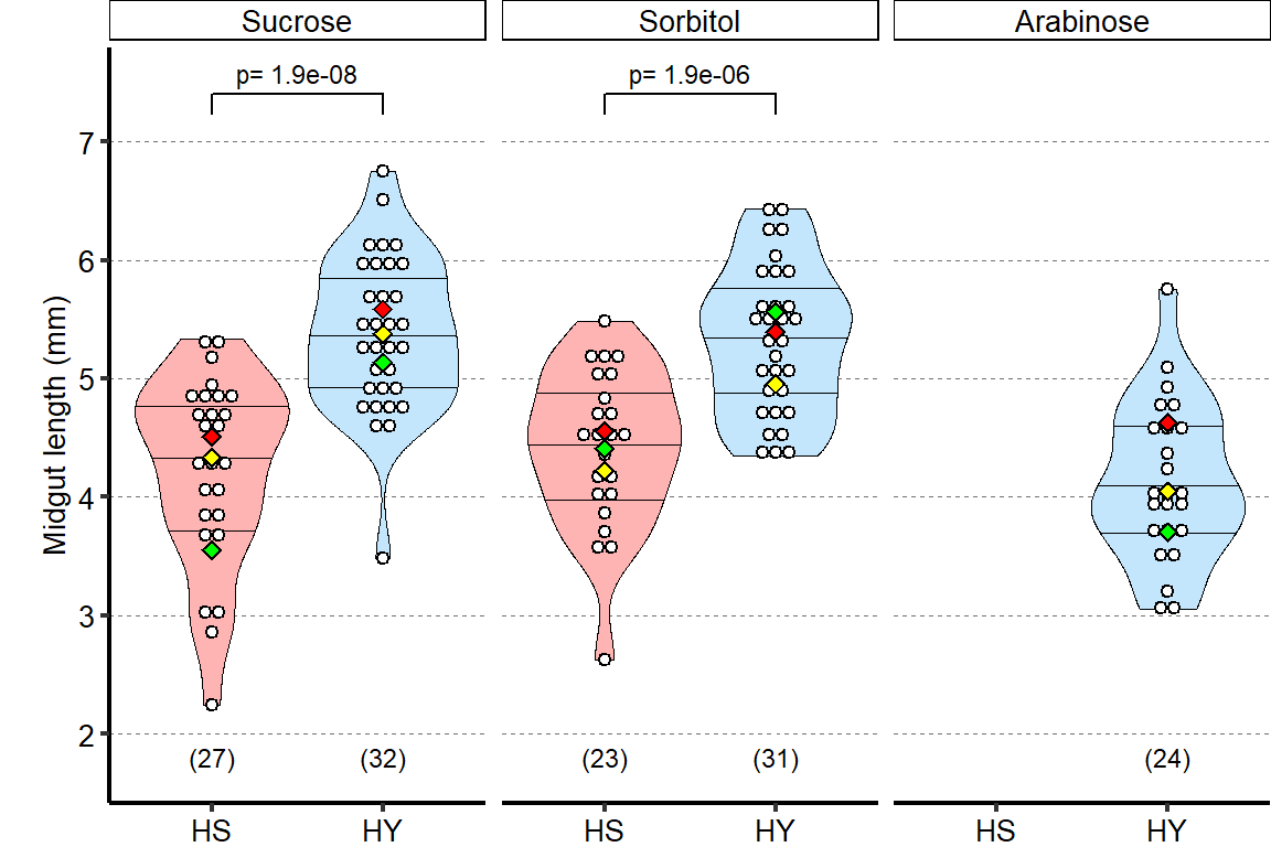
##Export Figure 2S2
3 Figure 3. Diet composition affects both cell number and enterocyte size in the midgut
3.1 Figure 3 - main
3.1.1 Figure 3A - B
Representative pictures of midguts from flies kept on HS (A) or HY (B) diet. Green arrows indicate intestinal stem cells (ISCs), marked only by GFP (green), red arrows mark enteroblasts (EBs), marked by GFP and GBE Su(H)-lacZ (red), and white arrow indicate enteroendocrine (EE) cells, marked with anti-Prospero antibody (white). All nuclei are stained with DAPI (blue). Complete graphical annotation can be found in manuscript figures
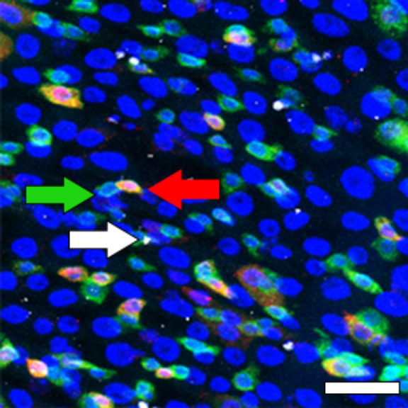
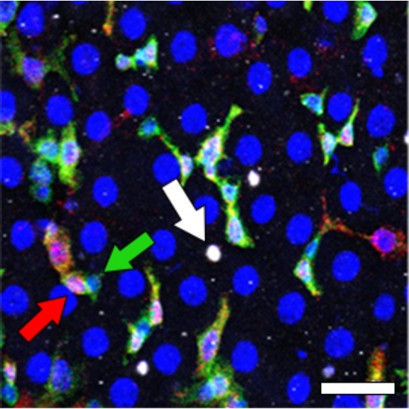
3.1.2 Figure 3C
Quantification of total cell numbers in the posterior midgut (R4) for HS and HY
Tab_cellnumber =
  d[["3C"]]%>%
     mutate(across(c(Diet,Line,Day,Repeat,GutNumber,Region),as.factor))%>%
     mutate(across(c(ISC.AL,EB.AL,EE.AL,EC.AL),round,0))

###Stats
#### ISC
mod.gen = fitme(log(ISC.AL) ~  Diet + (1 | Repeat), data = Tab_cellnumber)
shapiro.test(residuals(mod.gen))
    Shapiro-Wilk normality test

data:  residuals(mod.gen)
W = 0.96619, p-value = 0.01821bptest(log(ISC.AL) ~ Diet + (1 / Repeat), data = Tab_cellnumber)
    studentized Breusch-Pagan test

data:  log(ISC.AL) ~ Diet + (1/Repeat)
BP = 0.95685, df = 1, p-value = 0.328
mod.gen1 = fitme(log(ISC.AL) ~ 1 + (1 | Repeat), data = Tab_cellnumber)
test = anova(mod.gen, mod.gen1)
Chi2_LRT_growth = 2*(mod.gen$APHLs[["p_v"]]-mod.gen1$APHLs[["p_v"]])
tab_stat = data.frame(Comparison = as.character(paste("HS vs HY ISC")),
Cell_type = as.character(paste("ISC.AL")),
Rep = nlevels(Tab_cellnumber$Repeat),
chi2_LR = round(as.numeric(test$basicLRT$chi2_LR), digits = 2),
intercept = format(mod.gen$fixef[1],digits=3),
estimate = format(mod.gen$fixef[2],digits=3),
df = as.numeric(test$basicLRT$df),
Pvalue = as.numeric(format(pchisq(Chi2_LRT_growth,df=1,lower.tail = F),digits=2)))
tab_stat_ISC=tab_stat
#### EB
mod.gen = fitme(log(EB.AL) ~ Diet + (1 | Repeat),data = Tab_cellnumber)
shapiro.test(residuals(mod.gen))
    Shapiro-Wilk normality test

data:  residuals(mod.gen)
W = 0.98307, p-value = 0.2856bptest(log(EB.AL) ~ Diet + (1 / Repeat),data = Tab_cellnumber)
    studentized Breusch-Pagan test

data:  log(EB.AL) ~ Diet + (1/Repeat)
BP = 0.067845, df = 1, p-value = 0.7945
mod.gen1 = fitme(log(EB.AL) ~ 1 + (1 | Repeat), data = Tab_cellnumber)
test = anova(mod.gen, mod.gen1)
Chi2_LRT_growth = 2*(mod.gen$APHLs[["p_v"]]-mod.gen1$APHLs[["p_v"]])
tab_stat = data.frame(Comparison = as.character(paste("HS vs HY EB")),
Cell_type = as.character(paste("EB.AL")),
Rep = nlevels(Tab_cellnumber$Repeat),
chi2_LR = round(as.numeric(test$basicLRT$chi2_LR), digits = 2),
intercept = format(mod.gen$fixef[1],digits=3),
estimate = format(mod.gen$fixef[2],digits=3),
df = as.numeric(test$basicLRT$df),
Pvalue = as.numeric(format(pchisq(Chi2_LRT_growth,df=1,lower.tail = F),digits=2)))
tab_stat_EB=tab_stat
#### EC
mod.gen = fitme(log(EC.AL) ~ Diet + (1 | Repeat), data = Tab_cellnumber)
shapiro.test(residuals(mod.gen))
    Shapiro-Wilk normality test

data:  residuals(mod.gen)
W = 0.98161, p-value = 0.2211bptest(log(EC.AL) ~ Diet + (1 / Repeat), data = Tab_cellnumber)
    studentized Breusch-Pagan test

data:  log(EC.AL) ~ Diet + (1/Repeat)
BP = 1.7873, df = 1, p-value = 0.1813
mod.gen1 = fitme(log(EC.AL) ~ 1 + (1 | Repeat), data = Tab_cellnumber)
test = anova(mod.gen, mod.gen1)
test chi2_LR df p_value
p_v 37.74043 1 8.081226e-10Chi2_LRT_growth = 2*(mod.gen$APHLs[["p_v"]]-mod.gen1$APHLs[["p_v"]])
tab_stat = data.frame(Comparison = as.character(paste("HS vs HY EC")),
Cell_type = as.character(paste("EC.AL")),
Rep = nlevels(Tab_cellnumber$Repeat),
chi2_LR = round(as.numeric(test$basicLRT$chi2_LR), digits = 2),
intercept = format(mod.gen$fixef[1],digits=3),
estimate = format(mod.gen$fixef[2],digits=3),
df = as.numeric(test$basicLRT$df),
Pvalue = as.numeric(format(pchisq(Chi2_LRT_growth,df=1,lower.tail = F),digits=2)))
tab_stat_EC=tab_stat
#### EE
mod.gen = fitme(log(EE.AL) ~ Diet + (1 | Repeat), data = Tab_cellnumber)
shapiro.test(residuals(mod.gen))
    Shapiro-Wilk normality test

data:  residuals(mod.gen)
W = 0.97566, p-value = 0.08254bptest(log(EE.AL) ~ Diet + (1 / Repeat), data = Tab_cellnumber)
    studentized Breusch-Pagan test

data:  log(EE.AL) ~ Diet + (1/Repeat)
BP = 3.8518, df = 1, p-value = 0.04969
mod.gen1 = fitme(log(EE.AL) ~ 1 + (1 | Repeat), data = Tab_cellnumber)
test = anova(mod.gen, mod.gen1)
Chi2_LRT_growth = 2*(mod.gen$APHLs[["p_v"]]-mod.gen1$APHLs[["p_v"]])
tab_stat = data.frame(Comparison = as.character(paste("HS vs HY EE")),
Cell_type = as.character(paste("EE.AL")),
Rep = nlevels(Tab_cellnumber$Repeat),
chi2_LR = round(as.numeric(test$basicLRT$chi2_LR), digits = 2),
intercept = format(mod.gen$fixef[1],digits=3),
estimate = format(mod.gen$fixef[2],digits=3),
df = as.numeric(test$basicLRT$df),
Pvalue = as.numeric(format(pchisq(Chi2_LRT_growth,df=1,lower.tail = F),digits=2)))
tab_stat_EE=tab_stat
tab_stat=rbind(tab_stat_ISC,tab_stat_EB,tab_stat_EC,tab_stat_EE)
tab_stat$sig = ifelse(tab_stat$Pvalue < 0.05 & tab_stat$Pvalue > 0.01, "*",
ifelse(tab_stat$Pvalue < 0.01 & tab_stat$Pvalue > 0.001, "**",
ifelse(tab_stat$Pvalue < 0.001, "***", "")))
tab_stat%>%
kable(col.names = c("Comparison", "Cell type", "Replicates", "Chi2","Intercept","Estimate","df" ,"p-value","Signif."),row.names = FALSE) %>% add_header_above(c("log(Cell number) ~ Diet + (1 | Repeat)" = 9))%>%
kable_styling(bootstrap_options = c("striped", "hover", "condensed"), full_width = F)| Comparison | Cell type | Replicates | Chi2 | Intercept | Estimate | df | p-value | Signif. |
|---|---|---|---|---|---|---|---|---|
| HS vs HY ISC | ISC.AL | 6 | 16.77 | 6.25 | 0.425 | 1 | 4.2e-05 | *** |
| HS vs HY EB | EB.AL | 6 | 7.94 | 5.34 | 0.39 | 1 | 4.8e-03 | ** |
| HS vs HY EC | EC.AL | 6 | 37.74 | 7.62 | 0.374 | 1 | 0.0e+00 | *** |
| HS vs HY EE | EE.AL | 6 | 14.78 | 5.16 | 0.505 | 1 | 1.2e-04 | *** |
### Plot
Limits = c("HS", "HY")

Tab_cellnumber_gather=
  Tab_cellnumber %>%
  select(Diet,Line,Day,Repeat,GutNumber,Region,EB.AL,ISC.AL,EE.AL,EC.AL)%>%
  gather(key, value, -c(Diet,Line,Day,Repeat,GutNumber,Region)) %>%
  dplyr::rename(Cell_type = key,
         Cell_number = value) %>%
  mutate_if(is.character,as.factor)

Sample_size=
  subset(Tab_cellnumber_gather,!is.na(Day))%>%
  group_by(Diet,Cell_type)%>%
  summarise(Sample_size=n(),
            max=max(Cell_number,na.rm=T))

tmp=subset(Sample_size,Diet=="HY")
tab_stat =
  left_join(tab_stat,tmp)

Treatment.status = c("ISC", "EB","EC","EE")
names(Treatment.status) = c("ISC.AL", "EB.AL","EC.AL","EE.AL")


Plot_Fig3C=
  ggplot(Tab_cellnumber_gather, aes(x = Diet, y = Cell_number/100*2))+
  geom_violin(aes(fill = Diet), draw_quantiles = c(0.25, 0.5, 0.75), colour = "black", size = 0.2,adjust = 0.8) +
  geom_dotplot( colour = "black", fill = "white", binaxis = "y", stackdir = "center") +
  facet_wrap(.~Cell_type,scale="free_y",labeller=labeller(Cell_type=Treatment.status))+
  geom_blank(data=tab_stat, aes(y = max/100*2.5))+
  geom_signif(data = tab_stat, aes(xmin = 1, xmax = 2, annotations = formatC(paste("p=",Pvalue), digits = 2), y_position = max/100*2.2,), textsize = 3, vjust = -0.2, manual = TRUE)+
  scale_fill_manual(limits=Limits,
                    values=palette_diet_2)+
  scale_x_discrete("",
                   limits=c("HS", "HY"),
                   labels=c("HS (n = 46)", "HY (n = 55)"))+
  scale_y_continuous(expression(paste("Cell number in posterior midgut (x",10^2,")",sep="")))+
  stat_summary(fun = mean, geom = "point", size = 2.5, shape = 18, colour = "black", aes(group = Repeat)) +
                     stat_summary(fun = mean, geom = "point", size = 1.5, shape = 18, aes(group = Repeat, colour = Repeat)) +
                     scale_color_manual(values = palette_mean) +
  theme(
    panel.grid.major.y = element_line(colour = grey(0.45), linetype = "dashed", size = 0.2),
    panel.background = element_blank(),
    axis.title.x = element_text(size=Smallfont,colour="black"),
    axis.title.y = element_text(size=Smallfont,colour="black"),
    axis.line.x = element_line(colour="black",size=0.75),
    axis.line.y = element_line(colour="black",size=0.75),
    axis.ticks.x = element_line(size = 0.75),
    axis.ticks.y = element_line(size = 0.75),
    axis.text.x = element_text(size=Smallfont,colour="black",angle=30,hjust=1),
    axis.text.y = element_text(size=Smallfont,colour="black"),
    plot.margin = unit(Margin, "cm"),
    legend.direction = "vertical",
    legend.box = "horizontal",
    legend.position = "none",
    legend.key.height = unit(0.4, "cm"),
    legend.key.width= unit(0.6, "cm"),
    legend.title = element_text(face="italic",size=Smallfont),
    legend.key = element_rect(colour = 'white', fill = "white", linetype='dashed'),
    legend.text = element_text(size=SuperSmallfont),
    legend.background = element_rect(fill=NA),
    strip.text.x = element_text(size = Smallfont, colour = "black", margin = margin(t = 1, r = 0, b = 1, l = 0)),
    strip.text.y = element_text(size = Smallfont, colour = "black", margin = margin(t = 1, r = 0, b = 1, l = 0)),
    strip.background = element_rect(fill=NA, colour="black"),
    strip.placement="outside")

Plot_Fig3C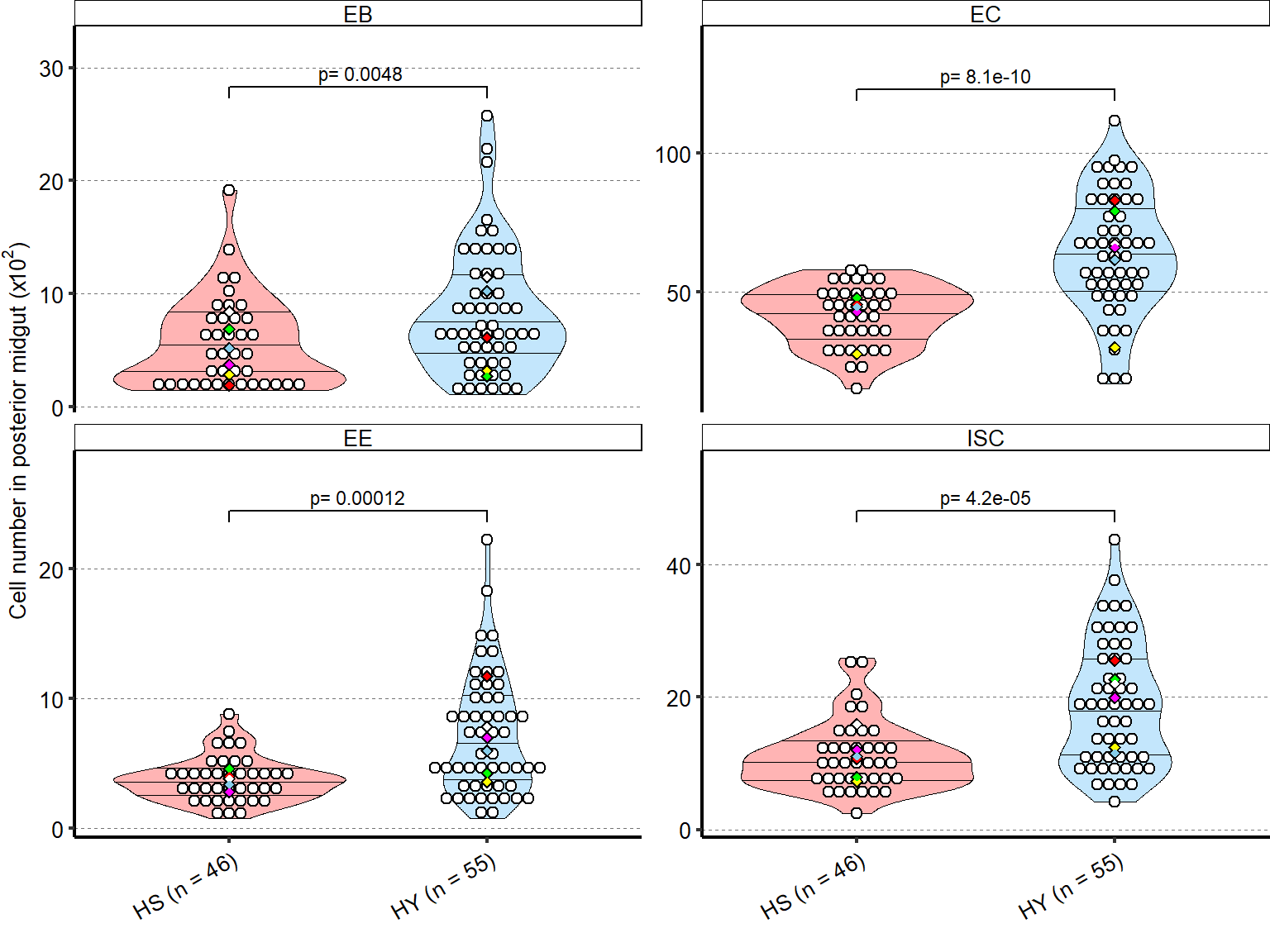
3.1.3 Figure 3D
HS and HY diets do not affect the relative proportion of cell types in the midgut (error is standard error of the mean).
tab_prop_cell_type =
  d[["3C"]]%>%
  dplyr::select(Diet, Line, Day, Repeat, GutNumber, Region | ends_with(".AL") & !starts_with("ESG"))%>%
  mutate_if(is.character,as.factor)%>%
  drop_na()%>%
  mutate(across(c(ISC.AL,EB.AL,EE.AL,EC.AL),round,0))%>%
  mutate(Total_cell=ISC.AL+EB.AL+EE.AL+EC.AL,
         proportion_ISC=ISC.AL/Total_cell*100,
         proportion_EB=EB.AL/Total_cell*100,
         proportion_EE=EE.AL/Total_cell*100,
         proportion_EC=EC.AL/Total_cell*100)%>%
  dplyr::select(Diet, Line, Day, Repeat, GutNumber, Region | starts_with("proportion"))%>%
  gather(key, value, -!starts_with("proportion") )%>%
  dplyr::rename(Cell_type = key,
         Cell_proportion = value) %>%
  mutate_if(is.character,as.factor) %>%
  group_by(Diet,Cell_type)%>%
  summarise(mean_proportion=mean(Cell_proportion, na.rm=T),
            se_proportion=se(Cell_proportion)) %>%
   as.data.frame()

for (i in 1:length(tab_prop_cell_type$se_proportion)){
    tab_prop_cell_type$se_proportionGraphPlus[i] = tab_prop_cell_type$mean_proportion[i]+tab_prop_cell_type$se_proportion[i]
    tab_prop_cell_type$se_proportionGraphMinus[i] = tab_prop_cell_type$mean_proportion[i]-tab_prop_cell_type$se_proportion[i]
}

for (i in 1:length(tab_prop_cell_type$se_proportion)){
  if(tab_prop_cell_type$Cell_type[i]=="proportion_EB"){
    tab_prop_cell_type$se_proportionGraphPlus[i] = tab_prop_cell_type$mean_proportion[i]+tab_prop_cell_type$se_proportion[i]

    tab_prop_cell_type$se_proportionGraphMinus[i] = tab_prop_cell_type$mean_proportion[i]-tab_prop_cell_type$se_proportion[i]

  }else{
    if(tab_prop_cell_type$Cell_type[i]=="proportion_EC"){

      tab_prop_cell_type$se_proportionGraphPlus[i] = tab_prop_cell_type$mean_proportion[i-1]+tab_prop_cell_type$mean_proportion[i]+tab_prop_cell_type$se_proportion[i]

      tab_prop_cell_type$se_proportionGraphMinus[i] = tab_prop_cell_type$mean_proportion[i-1]+tab_prop_cell_type$mean_proportion[i]+-tab_prop_cell_type$se_proportion[i]

    }else{
      if(tab_prop_cell_type$Cell_type[i]=="proportion_EE"){

        tab_prop_cell_type$se_proportionGraphPlus[i] =tab_prop_cell_type$mean_proportion[i-1]+ tab_prop_cell_type$mean_proportion[i-2]+tab_prop_cell_type$mean_proportion[i]+tab_prop_cell_type$se_proportion[i]

        tab_prop_cell_type$se_proportionGraphMinus[i] =tab_prop_cell_type$mean_proportion[i-1]+ tab_prop_cell_type$mean_proportion[i-2]+tab_prop_cell_type$mean_proportion[i]-tab_prop_cell_type$se_proportion[i]

      }else{
        tab_prop_cell_type$se_proportionGraphPlus[i] =tab_prop_cell_type$mean_proportion[i-1]+tab_prop_cell_type$mean_proportion[i-2]+ tab_prop_cell_type$mean_proportion[i-3]+tab_prop_cell_type$mean_proportion[i]+tab_prop_cell_type$se_proportion[i]

        tab_prop_cell_type$se_proportionGraphMinus[i] =tab_prop_cell_type$mean_proportion[i-1]+tab_prop_cell_type$mean_proportion[i-2]+ tab_prop_cell_type$mean_proportion[i-3]+tab_prop_cell_type$mean_proportion[i]-tab_prop_cell_type$se_proportion[i]
      }
    }
  }
}

tab_prop_cell_type$Cell_type =factor(tab_prop_cell_type$Cell_type,levels = c("proportion_ISC","proportion_EE","proportion_EC","proportion_EB"))

Plot_Fig3D =
ggplot(tab_prop_cell_type, aes(x=Diet, y=mean_proportion))+
  geom_bar(stat="identity",aes(fill=Cell_type),color="black",width=.90)+
  geom_errorbar(aes(ymin= se_proportionGraphMinus, ymax= se_proportionGraphPlus),width=0.25)+
  scale_fill_manual(name = "Cell types",
                    values=c("#1fd511","#ffffff", "#5869d5","#fe0000"),
                    labels = c("ISC", "EE", "EC","EB"))+
   scale_y_continuous("Proportion of cells (% \u00B1se)",
                      limits=c(0,101),
                      breaks=seq(0,100,by=25))+
  theme(
    panel.grid.major.y = element_line(colour = grey(0.45), linetype = "dashed", size = 0.2),
    panel.background = element_blank(),
    axis.title.x = element_blank(),
    axis.title.y = element_text(size=Smallfont,colour="black", hjust = 0.1 ),
    axis.line.x = element_line(colour="black",size=0.75),
    axis.line.y = element_line(colour="black",size=0.75),
    axis.ticks.x = element_line(size = 0.75),
    axis.ticks.y = element_line(size = 0.75),
    axis.text.x = element_text(size=Smallfont,colour="black"),
    axis.text.y = element_text(size=Smallfont,colour="black"),
    plot.margin = unit(Margin, "cm"),
    legend.direction = "vertical",
    legend.box = "horizontal",
    legend.position = "bottom",
    legend.key.height = unit(0.4, "cm"),
    legend.key.width= unit(0.6, "cm"),
    legend.title = element_text(face="italic",size=Smallfont),
    legend.key = element_rect(colour = 'white', fill = "white", linetype='dashed'),
    legend.text = element_text(size=Smallfont),
    legend.background = element_rect(fill=NA),
    strip.text.x = element_text(size =Smallfont, colour = "black",face="italic"),
    strip.text.y = element_text(size =Smallfont, colour = "black",face="italic"),
    strip.background = element_rect(fill=NA, colour="black"),
    strip.placement="outside")


Plot_Fig3D
3.1.4 Figure 3E - F
Diet affects enterocyte size. Representative picture of midguts stained with anti-Mesh antibody on HS (D, left) vs HY (E, right) diet. Complete graphical annotation can be found in manuscript figures
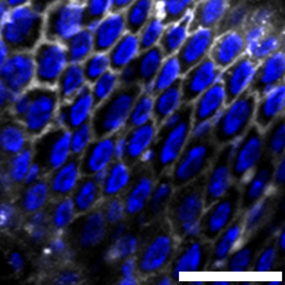

3.1.5 Figure 3G
Quantification of EC size of individuals on HS or HY diet for 5 days confirms an increase in cell size on HY diet.
tab_cell_area =
  d[["3G"]]%>%
  mutate_if(is.character,as.factor)%>%
  mutate_if(is.integer,as.factor)

Sample_size=
  tab_cell_area%>%
  group_by(Diet)%>%
  summarise(Sample_size=n())

###Stats

mod.gen = fitme(log(Area) ~  Diet + (1|Repeat),data =tab_cell_area)
shapiro.test(residuals(mod.gen))
    Shapiro-Wilk normality test

data:  residuals(mod.gen)
W = 0.99873, p-value = 0.5532bptest(log(Area) ~ Diet + (1/Repeat),data =tab_cell_area)
    studentized Breusch-Pagan test

data:  log(Area) ~ Diet + (1/Repeat)
BP = 14.735, df = 1, p-value = 0.0001237
mod.gen1 = fitme(log(Area) ~ 1 + (1|Repeat),data =tab_cell_area)
test = anova(mod.gen, mod.gen1)
Chi2_LRT_growth = 2*(mod.gen$APHLs[["p_v"]]-mod.gen1$APHLs[["p_v"]])
tab_stat = data.frame(Variable = as.character(paste("HS vs HY")),
Rep = nlevels(tab_cell_area$Repeat),
chi2_LR = round(as.numeric(test$basicLRT$chi2_LR), digits = 2),
intercept = format(mod.gen$fixef[1],digits=3),
estimate = format(mod.gen$fixef[2],digits=3),
df = as.numeric(test$basicLRT$df),
Pvalue = as.numeric(format(pchisq(Chi2_LRT_growth,df=1,lower.tail = F),digits=2)))
tab_stat$sig = ifelse(tab_stat$Pvalue < 0.05 & tab_stat$Pvalue > 0.01, "*",
ifelse(tab_stat$Pvalue < 0.01 & tab_stat$Pvalue > 0.001, "**",
ifelse(tab_stat$Pvalue < 0.001, "***", "")))
tab_stat%>%
kable(col.names = c("Comparison", "Replicates", "Chi2","Intercept","Estimate","df" ,"p-value","Signif."),row.names = FALSE) %>% add_header_above(c("log(Cell area) ~ Diet + (1 | Repeat)" = 8))%>%
kable_styling(bootstrap_options = c("striped", "hover", "condensed"), full_width = F)| Comparison | Replicates | Chi2 | Intercept | Estimate | df | p-value | Signif. |
|---|---|---|---|---|---|---|---|
| HS vs HY | 3 | 842.09 | 4.8 | 0.796 | 1 | 0 | *** |
### Plot

z = max(tab_cell_area$Area/1000, na.rm = TRUE)
Plot_Fig3G=
  ggplot(tab_cell_area, aes(x = Diet, y = Area/1000))+
  geom_violin(aes(fill = Diet), draw_quantiles = c(0.25, 0.5, 0.75), colour = "black", size = 0.2) +
  geom_dotplot( colour = "black", fill = "white", binaxis = "y", stackdir = "center", binwidth = z/140) +
  geom_text(data = Sample_size, mapping = aes(x = Diet, y = -0.01, label = paste("(",Sample_size,")",sep="")),size=3)+
 # geom_text(data = tab_stat, mapping = aes(x = 1.5, y = 0.62, label = paste("p=",format(Pvalue,digits=3))),size=3)+
    geom_signif(annotation = formatC(paste("p=",tab_stat$Pvalue), digits = 2), textsize = 3, y_position = 0.86, xmin = 1, xmax = 2, tip_length = c(0.02, 0.02), vjust = -0.2)+

  scale_fill_manual(limits=c("HS", "HY"),
                    values= palette_diet_2 )+
  scale_x_discrete("",
                   limits=c("HS", "HY"),
                   labels=c("HS", "HY"))+
  scale_y_continuous(expression(paste("EC area (10"^3, "mm"^2,")",sep="")),
                     limits=c(-0.01,0.9),
                     breaks=seq(0,0.8,by=0.1))+
  stat_summary(fun = mean, geom = "point", size = 3, shape = 18, colour = "black", aes(group = Repeat)) +
                     stat_summary(fun = mean, geom = "point", size = 2, shape = 18, aes(group = Repeat, colour = Repeat)) +
                     scale_color_manual(values = palette_mean) +
  theme(
    panel.grid.major.y = element_line(colour = grey(0.45), linetype = "dashed", size = 0.2),
    panel.background = element_blank(),
    axis.title.x = element_text(size=Smallfont,colour="black"),
    axis.title.y = element_text(size=Smallfont,colour="black"),
    axis.line.x = element_line(colour="black",size=0.75),
    axis.line.y = element_line(colour="black",size=0.75),
    axis.ticks.x = element_line(size = 0.75),
    axis.ticks.y = element_line(size = 0.75),
    axis.text.x = element_text(size=Smallfont,colour="black"),
    axis.text.y = element_text(size=Smallfont,colour="black"),
    plot.margin = unit(Margin, "cm"),
    legend.direction = "vertical",
    legend.box = "horizontal",
    legend.position = "none",
    legend.key.height = unit(0.4, "cm"),
    legend.key.width= unit(0.6, "cm"),
    legend.title = element_text(face="italic",size=Smallfont),
    legend.key = element_rect(colour = 'white', fill = "white", linetype='dashed'),
    legend.text = element_text(size=SuperSmallfont),
    legend.background = element_rect(fill=NA))

Plot_Fig3G
##Export Figure 3
3.2 Figure 3 - figure supplement 1
3.2.1 Figure 3S1A
ECs are more densely packed on HS diet than on HY diet.
tab_ECarea =
  d[["3C"]]%>%
  select(Diet, Line, Day, Repeat, GutNumber, Region,EC.A)%>%
  mutate_if(is.character,as.factor)%>%
  mutate_if(is.integer,as.factor)%>%
  dplyr::rename(EC_density=EC.A)%>%
  mutate(EC_density_mm=EC_density*1000)%>%
  drop_na()

Sample_size=
  tab_ECarea%>%
  group_by(Diet)%>%
  summarise(Sample_size=n())

###Stats

mod.gen = fitme(EC_density_mm ~  Diet + (1 | Repeat), data = tab_ECarea)
shapiro.test(residuals(mod.gen))
    Shapiro-Wilk normality test

data:  residuals(mod.gen)
W = 0.98248, p-value = 0.2538bptest(EC_density_mm ~ Diet + (1 / Repeat), data = tab_ECarea)
    studentized Breusch-Pagan test

data:  EC_density_mm ~ Diet + (1/Repeat)
BP = 0.027933, df = 1, p-value = 0.8673
mod.gen1 = fitme(EC_density_mm ~ 1 + (1 | Repeat), data = tab_ECarea)
test = anova(mod.gen, mod.gen1)
Chi2_LRT_growth = 2*(mod.gen$APHLs[["p_v"]]-mod.gen1$APHLs[["p_v"]])
#Now we make a tab with the results
tab_stat = data.frame(Variable = as.character(paste("HS vs HY")),
Rep = nlevels(tab_ECarea$Repeat),
chi2_LR = round(as.numeric(test$basicLRT$chi2_LR), digits = 2),
intercept = format(mod.gen$fixef[1],digits=3),
estimate = format(mod.gen$fixef[2],digits=3),
df = as.numeric(test$basicLRT$df),
Pvalue = as.numeric(format(pchisq(Chi2_LRT_growth,df=1,lower.tail = F),digits=2)))
tab_stat$sig = ifelse(tab_stat$Pvalue < 0.05 & tab_stat$Pvalue > 0.01, "*",
ifelse(tab_stat$Pvalue < 0.01 & tab_stat$Pvalue > 0.001, "**",
ifelse(tab_stat$Pvalue < 0.001, "***", "")))
tab_stat%>%
kable(col.names = c("Comparison", "Replicates", "Chi2","Intercept","Estimate","df" ,"p-value","Signif."),row.names = FALSE) %>% add_header_above(c("EC density ~ Diet + (1 | Repeat)" = 8))%>%
kable_styling(bootstrap_options = c("striped", "hover", "condensed"), full_width = F)| Comparison | Replicates | Chi2 | Intercept | Estimate | df | p-value | Signif. |
|---|---|---|---|---|---|---|---|
| HS vs HY | 6 | 20.79 | 5.98 | -1.18 | 1 | 5.1e-06 | *** |
Limits= c("HS","HY")

z=max(tab_ECarea$EC_density_mm, na.rm = TRUE)
Plot_Fig3S1A =
ggplot(tab_ECarea, aes(x=Diet, y=EC_density_mm))+
 geom_violin(aes(fill = Diet), draw_quantiles = c(0.25, 0.5, 0.75), colour = "black", size = 0.2,adjust = 0.8) +
  geom_dotplot( colour = "black", fill = "white", binaxis = "y", stackdir = "center", binwidth = z/60) +
  geom_text(data = Sample_size, mapping = aes(x = Diet, y = 1.8, label = paste("(",Sample_size,")",sep="")),size=3)+
    geom_signif(annotation = formatC(paste("p=",tab_stat$Pvalue), digits = 2), textsize = 3, y_position = 9, xmin = 1, xmax = 2, tip_length = c(0.02, 0.02), vjust = -0.2)+

  scale_fill_manual(limits=Limits,
                    values=palette_diet_2)+
  scale_x_discrete("",
                   limits=c("HS", "HY"),
                   labels=c("HS", "HY"))+
  scale_y_continuous(expression(paste("EC density (per ",mm^2,")")),
                     limits=c(1.5,9.5),
                     breaks=seq(2,8,by=1))+
      stat_summary(fun = mean, geom = "point", size = 3, shape = 18, colour = "black", aes(group = Repeat)) +
                     stat_summary(fun = mean, geom = "point", size = 2, shape = 18, aes(group = Repeat, colour = Repeat)) +
                     scale_color_manual(values = palette_mean) +
  theme(
    panel.grid.major.y = element_line(colour = grey(0.45), linetype = "dashed", size = 0.2),
    panel.background = element_blank(),
    axis.title.x = element_text(size=Smallfont,colour="black"),
    axis.title.y = element_text(size=Smallfont,colour="black"),
    axis.line.x = element_line(colour="black",size=0.75),
    axis.line.y = element_line(colour="black",size=0.75),
    axis.ticks.x = element_line(size = 0.75),
    axis.ticks.y = element_line(size = 0.75),
    axis.text.x = element_text(size=Smallfont,colour="black"),
    axis.text.y = element_text(size=Smallfont,colour="black"),
    plot.margin = unit(Margin, "cm"),
    legend.direction = "vertical",
    legend.box = "horizontal",
    legend.position = "none",
    legend.key.height = unit(0.4, "cm"),
    legend.key.width= unit(0.6, "cm"),
    legend.title = element_text(face="italic",size=Smallfont),
    legend.key = element_rect(colour = 'white', fill = "white", linetype='dashed'),
    legend.text = element_text(size=SuperSmallfont),
    legend.background = element_rect(fill=NA))

Plot_Fig3S1A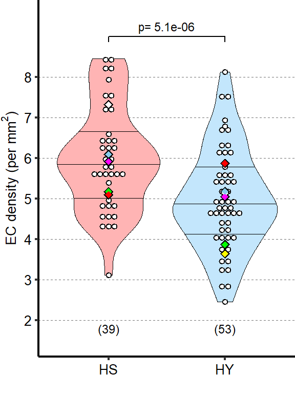
3.2.2 Figure 3S1B
Scheme illustrating area measurements. Top view in this scheme is as in pictures shown in figure 3 D, E. 3D side view show side view with Mesh showing measured surface.
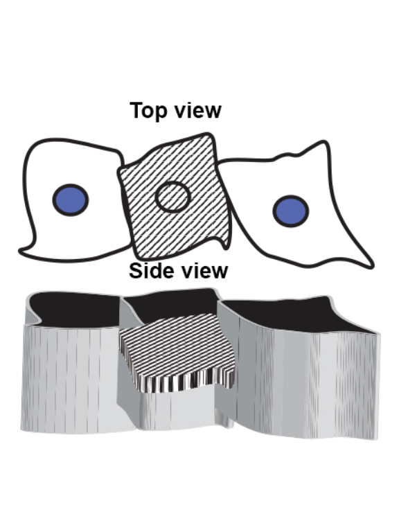
3.2.3 Figure 3S1C
Diet affects enterocyte size. Quantification of EC height of MyoTS>GFP on HS or HY diet demonstrates an increase in cell height on HY diet.
tab_ECheight =
  d[["3 - S1C"]]%>%
 select(Diet, Repeat, GutNumber, Region, Height)%>%
  mutate_if(is.character,as.factor)%>%
  mutate_if(is.integer,as.factor)%>%
  dplyr::rename(EC_height=Height)%>%
  drop_na()
tab_ECheight$EC_height <- as.numeric(tab_ECheight$EC_height)

Sample_size=
  tab_ECheight%>%
  group_by(Diet)%>%
  summarise(Sample_size=n())

###Stats

mod.gen = fitme((EC_height) ~  Diet + (1 | Repeat), data = tab_ECheight)
shapiro.test(residuals(mod.gen))
    Shapiro-Wilk normality test

data:  residuals(mod.gen)
W = 0.98665, p-value = 1.551e-06bptest(EC_height ~ Diet + (1 / Repeat), data = tab_ECheight)
    studentized Breusch-Pagan test

data:  EC_height ~ Diet + (1/Repeat)
BP = 40.813, df = 1, p-value = 1.676e-10
mod.gen1 = fitme(EC_height ~ 1 + (1 | Repeat), data = tab_ECheight)
test = anova(mod.gen, mod.gen1)
Chi2_LRT_growth = 2*(mod.gen$APHLs[["p_v"]]-mod.gen1$APHLs[["p_v"]])
#Now we make a tab with the results
tab_stat = data.frame(Variable = as.character(paste("HS vs HY")),
Rep = nlevels(tab_ECheight$Repeat),
chi2_LR = round(as.numeric(test$basicLRT$chi2_LR), digits = 2),
intercept = format(mod.gen$fixef[1],digits=3),
estimate = format(mod.gen$fixef[2],digits=3),
df = as.numeric(test$basicLRT$df),
Pvalue = as.numeric(format(pchisq(Chi2_LRT_growth,df=1,lower.tail = F),digits=2)))
tab_stat$sig = ifelse(tab_stat$Pvalue < 0.05 & tab_stat$Pvalue > 0.01, "*",
ifelse(tab_stat$Pvalue < 0.01 & tab_stat$Pvalue > 0.001, "**",
ifelse(tab_stat$Pvalue < 0.001, "***", "")))
tab_stat%>%
kable(col.names = c("Comparison", "Replicates", "Chi2","Intercept","Estimate","df" ,"p-value","Signif."),row.names = FALSE) %>% add_header_above(c("EC height ~ Diet + (1 | Repeat)" = 8))%>%
kable_styling(bootstrap_options = c("striped", "hover", "condensed"), full_width = F)| Comparison | Replicates | Chi2 | Intercept | Estimate | df | p-value | Signif. |
|---|---|---|---|---|---|---|---|
| HS vs HY | 2 | 494.51 | 7.09 | 5.03 | 1 | 0 | *** |
Limits= c("HS","HY")

z=max(tab_ECheight$EC_height, na.rm = TRUE)

Plot_Fig3S1C =
  ggplot(tab_ECheight, aes(x=Diet, y=EC_height))+
  geom_violin(aes(fill = Diet), draw_quantiles = c(0.25, 0.5, 0.75), colour = "black", size = 0.2,adjust = 0.8) +
  geom_dotplot( colour = "black", fill = "white", binaxis = "y", stackdir = "center", binwidth = z/150) +
  geom_text(data = Sample_size, mapping = aes(x = Diet, y = -1, label = paste("(",Sample_size,")",sep="")),size=3)+
    geom_signif(annotation = formatC(paste("p=",tab_stat$Pvalue), digits = 2), textsize = 3, y_position = 23, xmin = 1, xmax = 2, tip_length = c(0.02, 0.02), vjust = -0.2)+

  scale_fill_manual(limits=Limits,
                    values=palette_diet_2)+
  scale_x_discrete("",
                   limits=c("HS", "HY"),
                   labels=c("HS", "HY"))+
  scale_y_continuous(expression(paste("EC height (", mu, "m)")),
                     limits=c(-2,25),
                     breaks=seq(2,25,by=5))+
  stat_summary(fun = mean, geom = "point", size = 3, shape = 18, colour = "black", aes(group = Repeat)) +
  stat_summary(fun = mean, geom = "point", size = 2, shape = 18, aes(group = Repeat, colour = Repeat)) +
  scale_color_manual(values = palette_mean) +
  theme(
    panel.grid.major.y = element_line(colour = grey(0.45), linetype = "dashed", size = 0.2),
    panel.background = element_blank(),
    axis.title.x = element_text(size=Smallfont,colour="black"),
    axis.title.y = element_text(size=Smallfont,colour="black"),
    axis.line.x = element_line(colour="black",size=0.75),
    axis.line.y = element_line(colour="black",size=0.75),
    axis.ticks.x = element_line(size = 0.75),
    axis.ticks.y = element_line(size = 0.75),
    axis.text.x = element_text(size=Smallfont,colour="black"),
    axis.text.y = element_text(size=Smallfont,colour="black"),
    plot.margin = unit(Margin, "cm"),
    legend.direction = "vertical",
    legend.box = "horizontal",
    legend.position = "none",
    legend.key.height = unit(0.4, "cm"),
    legend.key.width= unit(0.6, "cm"),
    legend.title = element_text(face="italic",size=Smallfont),
    legend.key = element_rect(colour = 'white', fill = "white", linetype='dashed'),
    legend.text = element_text(size=SuperSmallfont),
    legend.background = element_rect(fill=NA))

Plot_Fig3S1C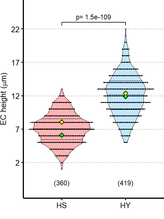
3.2.4 Figure 3S1D
Representative density plot from FACS for HS diet Complete annotation found in manuscript’s figures

3.2.5 Figure 3S1E
Representative density plot from FACS for HY diet Complete annotation found in manuscript’s figures
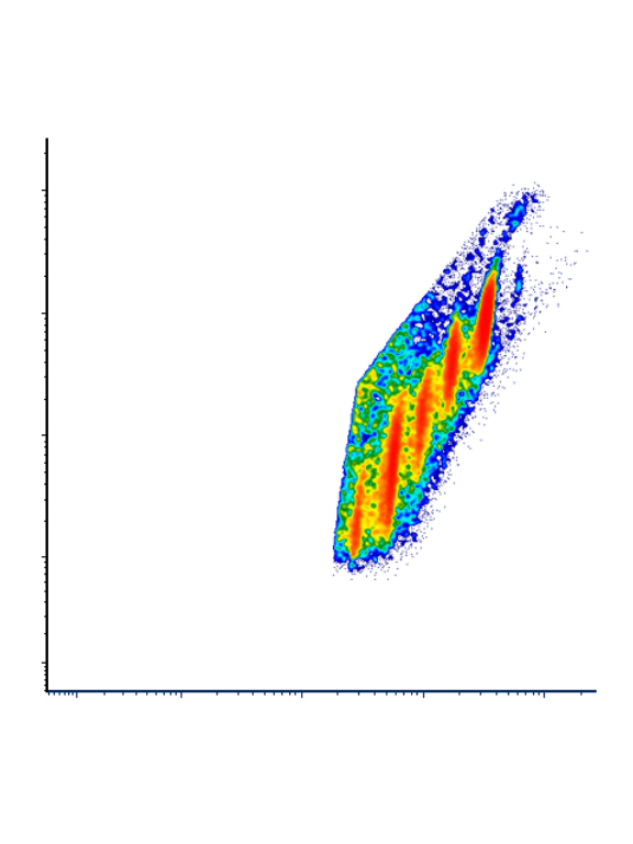
3.2.6 Figure 3S1F
Representative frequency plot from FACS for HS diet. Complete annotation found in manuscript’s figures

3.2.7 Figure 3S1G
Representative frequency plot from FACS for HY dietComplete annotation found in manuscript’s figures

3.2.8 Figure 3S1H
Ploidy of midguts on either HS or HY diets is largely unchanged. Stacked bar plot from 7 repeats, each of 25 midguts
tab_ploidy_rev =
  d[["3 - S1H"]]%>%
  mutate_if(is.character,as.factor)%>%
  mutate_if(is.integer,as.factor)%>%
  group_by(Diet, Ploidy)%>%
  summarise(mean_Percentage=mean(Percentage,na.rm=T),
            sd_Percentage=sd(Percentage))%>%
  mutate(group=paste(Diet, Ploidy,sep="_"))%>%
  mutate(Ploidy=fct_relevel(Ploidy,"2","4", "8", "16", "32", "64", "64+"))%>%
  as.data.frame()


Sample_size=
    tab_ploidy_rev%>%
  mutate_if(is.character,as.factor)%>%
  mutate_if(is.integer,as.factor)%>%
  group_by(Diet)%>%
  summarise(Sample_size=n())


# Creation of dataset with right position for error bar
##HS
tmp = subset(tab_ploidy_rev , Diet%in%c("HS"))


tmp1 <- subset(tmp, select = -c(group , sd_Percentage, Diet))


tmpw1 <-spread(tmp1, Ploidy, mean_Percentage)


tmpw1$`2.p` = tmpw1$`2`
tmpw1$`4.p` = tmpw1$`2` + tmpw1$`4`
tmpw1$`8.p` = tmpw1$`4.p` + tmpw1$`8`
tmpw1$`16.p` = tmpw1$`8.p` + tmpw1$`16`
tmpw1$`32.p` = tmpw1$`16.p` + tmpw1$`32`
tmpw1$`64.p` = tmpw1$`32.p` + tmpw1$`64`
tmpw1$`64+.p` = tmpw1$`64.p` + tmpw1$`64+`


tmp2 <- subset(tmp, select = -c(group , mean_Percentage, Diet))
tmpw2 <-spread(tmp2, Ploidy, sd_Percentage)

tmpw1$`2.se` = tmpw2$`2`
tmpw1$`4.se` = tmpw2$`4`
tmpw1$`8.se` = tmpw2$`8`
tmpw1$`16.se` = tmpw2$`16`
tmpw1$`32.se` = tmpw2$`32`
tmpw1$`64.se` = tmpw2$`64`
tmpw1$`64+.se` = tmpw2$`64+`


tmpw1$`2.se+` = tmpw1$`2` + tmpw1$`2.se`
tmpw1$`4.se+` = tmpw1$`4.p` + tmpw1$`4.se`
tmpw1$`8.se+` = tmpw1$`8.p` + tmpw1$`8.se`
tmpw1$`16.se+` = tmpw1$`16.p` + tmpw1$`16.se`
tmpw1$`32.se+` = tmpw1$`32.p` + tmpw1$`32.se`
tmpw1$`64.se+` = tmpw1$`64.p` + tmpw1$`64.se`
tmpw1$`64+.se+` = tmpw1$`64+.p` + tmpw1$`64+.se`


tmpw1$`2.se-` = tmpw1$`2` - tmpw1$`2.se`
tmpw1$`4.se-` = tmpw1$`4.p` - tmpw1$`4.se`
tmpw1$`8.se-` = tmpw1$`8.p` - tmpw1$`8.se`
tmpw1$`16.se-` = tmpw1$`16.p` - tmpw1$`16.se`
tmpw1$`32.se-` = tmpw1$`32.p` - tmpw1$`32.se`
tmpw1$`64.se-` = tmpw1$`64.p` - tmpw1$`64.se`
tmpw1$`64+.se-` = tmpw1$`64+.p` - tmpw1$`64+.se`


tmpl <- reshape(data=tmpw1,
    varying = list(Ploidy = c(1:7), Position = c(8:14), se = c(15:21), seplus = c(22:28), seminus = c(29:35)),
    direction = 'long',
    v.names = c("Percentage", "Position", "se", "seplus", "seminus"),
    sep = ".")

tmpl$Ploidy = c("2","4", "8", "16", "32", "64", "64+")

tmpl$Diet = "HS"


tmpl <- subset(tmpl, select = -c(time , id))

tmpl_HS <- tmpl

##HY
tmp = subset(tab_ploidy_rev , Diet%in%c("HY"))


tmp1 <- subset(tmp, select = -c(group , sd_Percentage, Diet))


tmpw1 <-spread(tmp1, Ploidy, mean_Percentage)


tmpw1$`2.p` = tmpw1$`2`
tmpw1$`4.p` = tmpw1$`2` + tmpw1$`4`
tmpw1$`8.p` = tmpw1$`4.p` + tmpw1$`8`
tmpw1$`16.p` = tmpw1$`8.p` + tmpw1$`16`
tmpw1$`32.p` = tmpw1$`16.p` + tmpw1$`32`
tmpw1$`64.p` = tmpw1$`32.p` + tmpw1$`64`
tmpw1$`64+.p` = tmpw1$`64.p` + tmpw1$`64+`


tmp2 <- subset(tmp, select = -c(group , mean_Percentage, Diet))
tmpw2 <-spread(tmp2, Ploidy, sd_Percentage)

tmpw1$`2.se` = tmpw2$`2`
tmpw1$`4.se` = tmpw2$`4`
tmpw1$`8.se` = tmpw2$`8`
tmpw1$`16.se` = tmpw2$`16`
tmpw1$`32.se` = tmpw2$`32`
tmpw1$`64.se` = tmpw2$`64`
tmpw1$`64+.se` = tmpw2$`64+`


tmpw1$`2.se+` = tmpw1$`2` + tmpw1$`2.se`
tmpw1$`4.se+` = tmpw1$`4.p` + tmpw1$`4.se`
tmpw1$`8.se+` = tmpw1$`8.p` + tmpw1$`8.se`
tmpw1$`16.se+` = tmpw1$`16.p` + tmpw1$`16.se`
tmpw1$`32.se+` = tmpw1$`32.p` + tmpw1$`32.se`
tmpw1$`64.se+` = tmpw1$`64.p` + tmpw1$`64.se`
tmpw1$`64+.se+` = tmpw1$`64+.p` + tmpw1$`64+.se`


tmpw1$`2.se-` = tmpw1$`2` - tmpw1$`2.se`
tmpw1$`4.se-` = tmpw1$`4.p` - tmpw1$`4.se`
tmpw1$`8.se-` = tmpw1$`8.p` - tmpw1$`8.se`
tmpw1$`16.se-` = tmpw1$`16.p` - tmpw1$`16.se`
tmpw1$`32.se-` = tmpw1$`32.p` - tmpw1$`32.se`
tmpw1$`64.se-` = tmpw1$`64.p` - tmpw1$`64.se`
tmpw1$`64+.se-` = tmpw1$`64+.p` - tmpw1$`64+.se`


tmpl <- reshape(data=tmpw1,
    varying = list(Ploidy = c(1:7), Position = c(8:14), se = c(15:21), seplus = c(22:28), seminus = c(29:35)),
    direction = 'long',
    v.names = c("Percentage", "Position", "se", "seplus", "seminus"),
    sep = ".")

tmpl$Ploidy = c("2","4", "8", "16", "32", "64", "64+")

tmpl$Diet = "HY"


tmpl <- subset(tmpl, select = -c(time , id))

tmpl_HY <- tmpl

#Bind, rename and reorcer
tab_ploidy <- rbind(tmpl_HS, tmpl_HY)
tab_ploidy$Ploidy <- as.factor(tab_ploidy$Ploidy)

tab_ploidy$Ploidy <-factor(tab_ploidy$Ploidy, levels =c("64+","64", "32", "16", "8", "4", "2"))

#Plot


Plot_Fig3S1H =
  ggplot(tab_ploidy, aes(x=Diet, y=Percentage))+
  geom_bar(stat="identity",aes(fill=Ploidy),color="black",width=.90)+
  geom_errorbar(aes(ymin= seminus, ymax= seplus),width=0.25, color = "black")+
  geom_text(data = Sample_size, mapping = aes(x = Diet, y = -5, label = paste("(",Sample_size,")",sep="")),size=3)+
  scale_fill_manual(name = "Ploidy",
                    values=c("#0052A2","#1A63AB", "#3375B5", "#6697C7", "#99BADA", "#CCDCEC", "#E6EEF6"),
                    labels = c("64+n", "64n", "32n", "16n", "8n", "4n", "2n"))+
  scale_y_continuous("Percentage of ploidy (mean \u00B1sd)",
                     limits=c(-5,90),
                     breaks=seq(0,80,by=20))+
  theme(
    panel.grid.major.y = element_line(colour = grey(0.45), linetype = "dashed", size = 0.2),
    panel.background = element_blank(),
    axis.title.x = element_blank(),
    axis.title.y = element_text(size=Smallfont,colour="black"),
    axis.line.x = element_line(colour="black",size=0.75),
    axis.line.y = element_line(colour="black",size=0.75),
    axis.ticks.x = element_line(size = 0.75),
    axis.ticks.y = element_line(size = 0.75),
    axis.text.x = element_text(size=Smallfont,colour="black"),
    axis.text.y = element_text(size=Smallfont,colour="black"),
    plot.margin = unit(Margin, "cm"),
    legend.direction = "horizontal",
    legend.box = "horizontal",
    legend.position = "bottom",
    #legend.key.height = unit(0.6, "cm"),
    #legend.key.width= unit(0.4, "cm"),
    legend.title = element_blank(),
    legend.key = element_rect(colour = 'white', fill = "white", linetype='dashed'),
    legend.text = element_text(size=Smallfont),
    legend.background = element_rect(fill=NA),
    strip.text = element_blank())+
    guides(fill=guide_legend(nrow=4,byrow=TRUE))

    #strip.background = element_rect(fill=NA, colour="black"),
    #strip.placement="outside")

Plot_Fig3S1H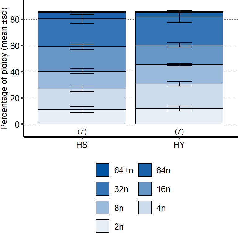
##Export Figure 3S1
4 Figure 4. Shifts in diet composition lead to plastic midgut resizing and changes in absolute and relative cell loss and gain
4.1 Figure 4 - main
4.1.1 Figure 4A
Midguts can respond plastically to changes in isocaloric diets. Midgut length increases from eclosion on HY for 7 days, then decreases when switched to HS for additional 7 days but can re-increase size upon a further 7 days HY feeding. Letters above violin plots represent grouping by statistical differences (Post hoc Tukey on GLMM).
Length_plasticity_time =
  d[["4A"]]%>%
  mutate_at(vars(starts_with("Total")),~./1000)%>%
  mutate_if(is.character,as.factor)%>%
  mutate_if(is.integer,as.factor)%>%
  dplyr::rename(Total_Length_mm=Total.L,
         Day_of_treatment=Day)

Sample_size=
  Length_plasticity_time%>%
  group_by(Diet)%>%
  summarise(Sample_size=n())

###Stats

mod.gen = fitme(log(Total_Length_mm) ~  Diet + (1 | Repeat), data = Length_plasticity_time)
shapiro.test(residuals(mod.gen))
    Shapiro-Wilk normality test

data:  residuals(mod.gen)
W = 0.99167, p-value = 0.7868bptest(log(Total_Length_mm) ~ Diet + (1 / Repeat), data = Length_plasticity_time)
    studentized Breusch-Pagan test

data:  log(Total_Length_mm) ~ Diet + (1/Repeat)
BP = 12.435, df = 3, p-value = 0.006032
mod.gen1 = fitme(log(Total_Length_mm) ~ 1 + (1 | Repeat), data = Length_plasticity_time)
test = anova(mod.gen, mod.gen1)
Chi2_LRT_growth = 2*(mod.gen$APHLs[["p_v"]]-mod.gen1$APHLs[["p_v"]])
tab_stat = data.frame(Variable = as.character(paste("Anova diets")),
Rep = nlevels(Length_plasticity_time$Repeat),
chi2_LR = round(as.numeric(test$basicLRT$chi2_LR), digits = 2),
intercept = format(mod.gen$fixef[1],digits=3),
estimate = format(mod.gen$fixef[2],digits=3),
df = as.numeric(test$basicLRT$df),
Pvalue = as.numeric(format(pchisq(Chi2_LRT_growth,df=1,lower.tail = F),digits=2)))
tab_stat$sig = ifelse(tab_stat$Pvalue < 0.05 & tab_stat$Pvalue > 0.01, "*",
ifelse(tab_stat$Pvalue < 0.01 & tab_stat$Pvalue > 0.001, "**",
ifelse(tab_stat$Pvalue < 0.001, "***", "")))
tab_stat%>%
kable(col.names = c("Comparison", "Replicates", "Chi2","Intercept","Estimate","df" ,"p-value","Signif."),row.names = FALSE) %>% add_header_above(c("log(Total_Length_mm) ~ Diet + (1 | Repeat)" = 8))%>%
kable_styling(bootstrap_options = c("striped", "hover", "condensed"), full_width = F)| Comparison | Replicates | Chi2 | Intercept | Estimate | df | p-value | Signif. |
|---|---|---|---|---|---|---|---|
| Anova diets | 3 | 106.66 | 1.22 | 0.553 | 3 | 0 | *** |
mod.gen = lmer(log(Total_Length_mm) ~  Diet + (1 | Repeat), data = Length_plasticity_time)
multcomp = glht(mod.gen, linfct=mcp(Diet="Tukey"))

tmp = cld(multcomp)

letter_position = aggregate(data=Length_plasticity_time,Total_Length_mm ~  Diet, max)

tab_letter =  as.data.frame(tmp$mcletters$Letters)
tab_letter$Diet=rownames(tab_letter)
colnames(tab_letter)[1] = "Letter"
tab_letter = left_join(tab_letter,letter_position)

### Plot
Limits = c("Eclosion","HY","HYtoHS", "HYtoHStoHY")
z = max(Length_plasticity_time$Total_Length_mm, na.rm = TRUE)

Plot_Fig4A=
  ggplot(Length_plasticity_time, aes(x = Diet, y = Total_Length_mm))+
  geom_violin(aes(fill = Diet), draw_quantiles = c(0.25, 0.5, 0.75), colour = "black", size = 0.2,adjust = 0.8) +
  geom_dotplot( colour = "black", fill = "white", binaxis = "y", stackdir = "center", binwidth = z/60) +
  geom_text(data = Sample_size, mapping = aes(x = Diet, y = 1.5, label = paste("(",Sample_size,")",sep="")),size=3)+
geom_text(data = tab_letter, mapping = aes(x = Diet, y = Total_Length_mm+0.4, label = Letter),size=3)+
  geom_text(data = tab_stat, mapping = aes(x = 1.2, y = 7.5, label = paste("p=",format(Pvalue,digits=2))),size=3)+
  scale_fill_manual(limits=Limits,
                    values=cbbPalette_4)+
  scale_x_discrete("",
                   limits=Limits,
                   labels=c("Eclosion","HY","HY to HS", "HY to HS to HY"))+
  scale_y_continuous("Midgut length (mm)",
                     limits=c(1.3,8.2),
                     breaks=seq(2,8,by=1),
                     minor_breaks = seq(3, 7,by= 1))+
  stat_summary(fun = mean, geom = "point", size = 3, shape = 18, colour = "black", aes(group = Repeat)) +
                     stat_summary(fun = mean, geom = "point", size = 2, shape = 18, aes(group = Repeat, colour = Repeat)) +
                     scale_color_manual(values = palette_mean) +
  theme(panel.grid.major.y = element_line(colour = grey(0.45), linetype = "dashed", size = 0.2),
        panel.background = element_blank(),
        axis.title.x = element_text(size=Smallfont,colour="black"),
        axis.title.y = element_text(size=Smallfont,colour="black"),
        axis.line.x = element_line(colour="black",size=0.75),
        axis.line.y = element_line(colour="black",size=0.75),
        axis.ticks.x = element_line(size = 0.75),
        axis.ticks.y = element_line(size = 0.75),
        axis.text.x = element_text(size=Smallfont,colour="black",angle=30,hjust=1),
        axis.text.y = element_text(size=Smallfont,colour="black"),
        plot.margin = unit(Margin, "cm"),
        legend.direction = "vertical",
        legend.box = "horizontal",
        legend.position = "none",
        legend.key.height = unit(0.4, "cm"),
        legend.key.width= unit(0.6, "cm"),
        legend.title = element_text(face="italic",size=Smallfont),
        legend.key = element_rect(colour = 'white', fill = "white", linetype='dashed'),
        legend.text = element_text(size=SuperSmallfont),
        legend.background = element_rect(fill=NA),
        strip.text.x = element_text(size =Smallfont, colour = "black",face="italic"),
        strip.text.y = element_text(size =Smallfont, colour = "black",face="italic"),
        strip.background = element_rect(fill=NA, colour="black"),
        strip.placement="outside")

Plot_Fig4A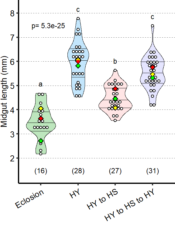
4.1.2 Figure 4B
Mitotically active cells visualized by phospho-Histone H3 (pH3) immunostaining are more numerous on HY diet than on HS diet. pH3+ cells gradually increase over time on HY, but not HS diet. Letters above violin plots represent grouping by statistical differences (Post hoc Tukey on GLMM).
Length_Diet_time =
  d[["4B, 4S1C"]]%>%
  mutate_at(vars(ends_with(".L")),~./1000)%>%
  mutate_at(vars(!starts_with("Total")),as.factor)%>%
  mutate(group=paste(Diet, Day,sep="_"))%>%
 dplyr::rename(Total_Length_mm=Total.L,
         PH3_positive_cell=Total.PH3,
         Day_of_treatment=Day)

Sample_size=
  Length_Diet_time%>%
  group_by(Diet,Day_of_treatment)%>%
  summarise(Sample_size=n())

###Stats

mod.gen = fitme(PH3_positive_cell ~  group + (1 | Repeat),data = subset(Length_Diet_time,!is.na(PH3_positive_cell)))
shapiro.test(residuals(mod.gen))
    Shapiro-Wilk normality test

data:  residuals(mod.gen)
W = 0.97954, p-value = 0.01115bptest(PH3_positive_cell ~ group + (1 / Repeat),data = subset(Length_Diet_time,!is.na(PH3_positive_cell)))
    studentized Breusch-Pagan test

data:  PH3_positive_cell ~ group + (1/Repeat)
BP = 41.055, df = 7, p-value = 7.901e-07
mod.gen1 = fitme(PH3_positive_cell ~ 1 + (1 | Repeat),data = subset(Length_Diet_time,!is.na(PH3_positive_cell)))
test = anova(mod.gen, mod.gen1)
Chi2_LRT_growth = 2*(mod.gen$APHLs[["p_v"]]-mod.gen1$APHLs[["p_v"]])
tab_stat = data.frame(Variable = as.character(paste("Any difference")),
Rep = nlevels(Length_Diet_time$Repeat),
chi2_LR = round(as.numeric(test$basicLRT$chi2_LR), digits = 2),
intercept = format(mod.gen$fixef[1],digits=3),
estimate = format(mod.gen$fixef[2],digits=3),
df = as.numeric(test$basicLRT$df),
Pvalue = as.numeric(format(pchisq(Chi2_LRT_growth,df=1,lower.tail = F),digits=2)))
tab_stat$sig = ifelse(tab_stat$Pvalue < 0.05 & tab_stat$Pvalue > 0.01, "*",
ifelse(tab_stat$Pvalue < 0.01 & tab_stat$Pvalue > 0.001, "**",
ifelse(tab_stat$Pvalue < 0.001, "***", "")))
tab_stat%>%
kable(col.names = c("Comparison", "Replicates", "Chi2","Intercept","Estimate","df" ,"p-value","Signif."),row.names = FALSE) %>% add_header_above(c("PH3_positive_cell ~ group + (1 | Repeat)" = 8))%>%
kable_styling(bootstrap_options = c("striped", "hover", "condensed"), full_width = F)| Comparison | Replicates | Chi2 | Intercept | Estimate | df | p-value | Signif. |
|---|---|---|---|---|---|---|---|
| Any difference | 3 | 248.1 | 11.4 | 3.98 | 7 | 0 | *** |
tab_stat$Diet="HS"

mod.gen = lmer(PH3_positive_cell ~  group + (1 | Repeat),data =subset(Length_Diet_time,!is.na(PH3_positive_cell)))
multcomp = glht(mod.gen, linfct=mcp(group="Tukey"))

tmp = cld(multcomp)

letter_position = aggregate(data=subset(Length_Diet_time,!is.na(PH3_positive_cell)),PH3_positive_cell ~  group, max)

tab_letter =  as.data.frame(tmp$mcletters$Letters)
tab_letter$group=rownames(tab_letter)
colnames(tab_letter)[1] = "Letter"
tab_letter = left_join(tab_letter,letter_position)
tab_letter = separate(tab_letter,group, c("Diet", "Day_of_treatment"), sep = "_", remove=FALSE)

### Plot
Limits = c("7","14","21", "28")
z = max(Length_Diet_time$PH3_positive_cell, na.rm = TRUE)

Plot_Fig4B=
  ggplot(Length_Diet_time, aes(x = Day_of_treatment, y = PH3_positive_cell))+
  geom_violin(aes(fill = Diet), draw_quantiles = c(0.25, 0.5, 0.75), colour = "black", size = 0.2,adjust = 0.8) +
  geom_dotplot( colour = "black", fill = "white", binaxis = "y", stackdir = "center", binwidth = z/40) +
  facet_grid(. ~ Diet)+
  geom_text(data = Sample_size, mapping = aes(x = Day_of_treatment, y = -8, label = paste("(",Sample_size,")",sep="")),size=3)+
  geom_text(data = tab_letter, mapping = aes(x = Day_of_treatment, y = PH3_positive_cell+10, label = Letter),size=3)+
  geom_text(data = tab_stat, mapping = aes(x = 2, y = 130, label = paste("p=",format(Pvalue,digits=2))),size=3)+
   scale_fill_manual(limits=c("HS","HY"),
                     values=palette_diet_2)+
  scale_x_discrete("",
                   limits=Limits,
                   labels=c("7 days","14 days", "21 days", "28 days"))+
  scale_y_continuous(expression(paste("pH3" ^ "+", " cells")),
                     limits=c(-10,140),
                     breaks=seq(0,140,by=20))+
     stat_summary(fun = mean, geom = "point", size = 3, shape = 18, colour = "black", aes(group = Repeat)) +
                     stat_summary(fun = mean, geom = "point", size = 2, shape = 18, aes(group = Repeat, colour = Repeat)) +
                     scale_color_manual(values = palette_mean) +
  theme(panel.grid.major.y = element_line(colour = grey(0.45), linetype = "dashed", size = 0.2),
        panel.background = element_blank(),
        axis.title.x = element_text(size=Smallfont,colour="black"),
        axis.title.y = element_text(size=Smallfont,colour="black"),
        axis.line.x = element_line(colour="black",size=0.75),
        axis.line.y = element_line(colour="black",size=0.75),
        axis.ticks.x = element_line(size = 0.75),
        axis.ticks.y = element_line(size = 0.75),
        axis.text.x = element_text(size=Smallfont,colour="black",angle=30,hjust=1),
        axis.text.y = element_text(size=Smallfont,colour="black"),
        plot.margin = unit(Margin, "cm"),
        legend.direction = "vertical",
        legend.box = "horizontal",
        legend.position = "none",
        legend.key.height = unit(0.4, "cm"),
        legend.key.width= unit(0.6, "cm"),
        legend.title = element_text(face="italic",size=Smallfont),
        legend.key = element_rect(colour = 'white', fill = "white", linetype='dashed'),
        legend.text = element_text(size=SuperSmallfont),
        legend.background = element_rect(fill=NA),
        strip.text.x = element_text(size = Smallfont, colour = "black", margin = margin(t = 2, r = 0, b = 2, l = 0)),
        strip.text.y = element_text(size = Smallfont, colour = "black", margin = margin(t = 2, r = 0, b = 2, l = 0)),
        strip.background = element_rect(fill=NA, colour="black"),
        strip.placement="outside")

Plot_Fig4B
4.1.3 Figure 4C
Shifting between diets impacts pH3+ cell number in growth (HS to HY) experiments. Statistical comparisons are vs pre-shift measurement.
Length_Growth_PH3 =
  d[["4C, 4S1D"]]%>%
  mutate_at(vars(ends_with(".L")),~./1000)%>%
  mutate_at(vars(!starts_with("Total")),as.factor)%>%
  dplyr::rename(Total_Length_mm=Total.L,
         PH3_positive_cell=Total.PH3,
         Day_of_treatment=Day)%>%
  as.data.frame()%>%
  mutate(Dday=fct_relevel(Dday,"Shift Day 7","Shift Day 14","Shift Day 21"))

Sample_size=
  Length_Growth_PH3%>%
  group_by(Diet,Dday)%>%
  summarise(Sample_size=n())

###Stats
###Day 7
mod.gen = fitme(log(PH3_positive_cell) ~  Diet + (1 | Repeat),data = subset(Length_Growth_PH3,Dday=="Shift Day 7"))
shapiro.test(residuals(mod.gen))
    Shapiro-Wilk normality test

data:  residuals(mod.gen)
W = 0.97011, p-value = 0.2797bptest(log(PH3_positive_cell) ~ Diet + (1 / Repeat),data = subset(Length_Growth_PH3,Dday=="Shift Day 7"))
    studentized Breusch-Pagan test

data:  log(PH3_positive_cell) ~ Diet + (1/Repeat)
BP = 1.8138, df = 1, p-value = 0.1781
mod.gen1 = fitme(log(PH3_positive_cell) ~ 1 + (1 | Repeat),data = subset(Length_Growth_PH3,Dday=="Shift Day 7"))
test = anova(mod.gen, mod.gen1)
Chi2_LRT_growth = 2*(mod.gen$APHLs[["p_v"]]-mod.gen1$APHLs[["p_v"]])
tab_stat = data.frame(Comparison = as.character(paste("HS Day 7 vs HS to HY Day 14")),
Variable = as.character(paste("Shift Day 7")),
Rep = nlevels(Length_Growth_PH3$Repeat),
chi2_LR = round(as.numeric(test$basicLRT$chi2_LR), digits = 2),
intercept = format(mod.gen$fixef[1],digits=3),
estimate = format(mod.gen$fixef[2],digits=3),
df = as.numeric(test$basicLRT$df),
Pvalue = as.numeric(format(pchisq(Chi2_LRT_growth,df=1,lower.tail = F),digits=2)))
tab_stat_7=tab_stat
#Day 14
mod.gen = fitme(log(PH3_positive_cell) ~ Diet + (1 | Repeat),data = subset(Length_Growth_PH3,Dday=="Shift Day 14"))
shapiro.test(residuals(mod.gen))
    Shapiro-Wilk normality test

data:  residuals(mod.gen)
W = 0.95426, p-value = 0.1063bptest(log(PH3_positive_cell) ~ Diet + (1 / Repeat),data = subset(Length_Growth_PH3,Dday=="Shift Day 14"))
    studentized Breusch-Pagan test

data:  log(PH3_positive_cell) ~ Diet + (1/Repeat)
BP = 0.20868, df = 1, p-value = 0.6478
mod.gen1 = fitme(log(PH3_positive_cell) ~ 1 + (1 | Repeat),data = subset(Length_Growth_PH3,Dday=="Shift Day 14"))
test = anova(mod.gen, mod.gen1)
Chi2_LRT_growth = 2*(mod.gen$APHLs[["p_v"]]-mod.gen1$APHLs[["p_v"]])
tab_stat = data.frame(Comparison = as.character(paste("HS Day 14 vs HS to HY Day 21")),
Variable = as.character(paste("Shift Day 14")),
Rep = nlevels(Length_Growth_PH3$Repeat),
chi2_LR = round(as.numeric(test$basicLRT$chi2_LR), digits = 2),
intercept = format(mod.gen$fixef[1],digits=3),
estimate = format(mod.gen$fixef[2],digits=3),
df = as.numeric(test$basicLRT$df),
Pvalue = as.numeric(format(pchisq(Chi2_LRT_growth,df=1,lower.tail = F),digits=2)))
tab_stat_14=tab_stat
#Day 21
mod.gen = fitme(log(PH3_positive_cell) ~ Diet + (1 | Repeat),data = subset(Length_Growth_PH3,Dday=="Shift Day 21"))
shapiro.test(residuals(mod.gen))
    Shapiro-Wilk normality test

data:  residuals(mod.gen)
W = 0.93625, p-value = 0.005926bptest(log(PH3_positive_cell) ~ Diet + (1 / Repeat),data = subset(Length_Growth_PH3,Dday=="Shift Day 21"))
    studentized Breusch-Pagan test

data:  log(PH3_positive_cell) ~ Diet + (1/Repeat)
BP = 1.3963, df = 1, p-value = 0.2373
mod.gen1 = fitme(log(PH3_positive_cell) ~ 1 + (1 | Repeat),data = subset(Length_Growth_PH3,Dday=="Shift Day 21"))
test = anova(mod.gen, mod.gen1)
Chi2_LRT_growth = 2*(mod.gen$APHLs[["p_v"]]-mod.gen1$APHLs[["p_v"]])
tab_stat = data.frame(Comparison = as.character(paste("HS Day 21 vs HS to HY Day 28")),
Variable = as.character(paste("Shift Day 21")),
Rep = nlevels(Length_Growth_PH3$Repeat),
chi2_LR = round(as.numeric(test$basicLRT$chi2_LR), digits = 2),
intercept = format(mod.gen$fixef[1],digits=3),
estimate = format(mod.gen$fixef[2],digits=3),
df = as.numeric(test$basicLRT$df),
Pvalue = as.numeric(format(pchisq(Chi2_LRT_growth,df=1,lower.tail = F),digits=2)))
tab_stat_21 = tab_stat
tab_stat=rbind(tab_stat_7,tab_stat_14,tab_stat_21)
tab_stat$sig = ifelse(tab_stat$Pvalue < 0.05 & tab_stat$Pvalue > 0.01, "*",
ifelse(tab_stat$Pvalue < 0.01 & tab_stat$Pvalue > 0.001, "**",
ifelse(tab_stat$Pvalue < 0.001, "***", "")))
tab_stat%>%
kable(col.names = c("Comparison", "Variable", "Replicates", "Chi2","Intercept","Estimate","df" ,"p-value","Signif."),row.names = FALSE) %>% add_header_above(c("log(PH3_positive_cell) ~ Diet + (1 | Repeat)" = 9))%>%
kable_styling(bootstrap_options = c("striped", "hover", "condensed"), full_width = F)| Comparison | Variable | Replicates | Chi2 | Intercept | Estimate | df | p-value | Signif. |
|---|---|---|---|---|---|---|---|---|
| HS Day 7 vs HS to HY Day 14 | Shift Day 7 | 3 | 28.80 | 2.07 | 1.38 | 1 | 1e-07 | *** |
| HS Day 14 vs HS to HY Day 21 | Shift Day 14 | 3 | 24.15 | 2.26 | 1.12 | 1 | 9e-07 | *** |
| HS Day 21 vs HS to HY Day 28 | Shift Day 21 | 3 | 45.01 | 2.57 | 1.29 | 1 | 0e+00 | *** |
tab_stat=
  tab_stat %>%
  dplyr::rename(Dday=Variable)%>%
  as.data.frame()%>%
  mutate(Dday=fct_relevel(Dday,"Shift Day 7","Shift Day 14","Shift Day 21"))

### Plot
Limits = c("HS","HStoHY")
z=max(Length_Growth_PH3$PH3_positive_cell, na.rm = TRUE)

Plot_Fig4C=
  ggplot(Length_Growth_PH3, aes(x = Diet, y = PH3_positive_cell))+
  geom_violin(aes(fill = Diet), draw_quantiles = c(0.25, 0.5, 0.75), colour = "black", size = 0.2,adjust = 0.8) +
  geom_dotplot( colour = "black", fill = "white", binaxis = "y", stackdir = "center", binwidth = z/40) +
  facet_grid(. ~ Dday)+
  geom_text(data = Sample_size, mapping = aes(x = Diet, y = -5, label = paste("(",Sample_size,")",sep="")),size=3)+
    geom_signif(data = tab_stat, aes(xmin = 1, xmax = 2, annotations = formatC(paste("p=",Pvalue), digits = 2), y_position = 132,), textsize = 3, vjust = -0.2, manual = TRUE)+

  scale_fill_manual(limits=c("HS","HStoHY"),
                    values=cbbHS_HStoHY)+
  scale_x_discrete("",
                   limits=Limits,
                   labels=c("HS","HS to HY"))+
  scale_y_continuous(expression(paste("pH3" ^ "+", " cells")),
                     limits=c(-8,136),
                     breaks=seq(0,120,by=20))+
stat_summary(fun = mean, geom = "point", size = 3, shape = 18, colour = "black", aes(group = Repeat)) +
                     stat_summary(fun = mean, geom = "point", size = 2, shape = 18, aes(group = Repeat, colour = Repeat)) +
                     scale_color_manual(values = palette_mean) +
  theme(panel.grid.major.y = element_line(colour = grey(0.45), linetype = "dashed", size = 0.2),
        panel.background = element_blank(),
        axis.title.x = element_text(size=Smallfont,colour="black"),
        axis.title.y = element_text(size=Smallfont,colour="black"),
        axis.line.x = element_line(colour="black",size=0.75),
        axis.line.y = element_line(colour="black",size=0.75),
        axis.ticks.x = element_line(size = 0.75),
        axis.ticks.y = element_line(size = 0.75),
        axis.text.x = element_text(size=Smallfont,colour="black",angle=30,hjust=1),
        axis.text.y = element_text(size=Smallfont,colour="black"),
        plot.margin = unit(Margin, "cm"),
        legend.direction = "vertical",
        legend.box = "horizontal",
        legend.position = "none",
        legend.key.height = unit(0.4, "cm"),
        legend.key.width= unit(0.6, "cm"),
        legend.title = element_text(face="italic",size=Smallfont),
        legend.key = element_rect(colour = 'white', fill = "white", linetype='dashed'),
        legend.text = element_text(size=SuperSmallfont),
        legend.background = element_rect(fill=NA),
            strip.text.x = element_text(size = Smallfont, colour = "black", margin = margin(t = 2, r = 0, b = 2, l = 0)),
        strip.text.y = element_text(size = Smallfont, colour = "black", margin = margin(t = 2, r = 0, b = 2, l = 0)),
        strip.background = element_rect(fill=NA, colour="black"),
        strip.placement="outside")

Plot_Fig4C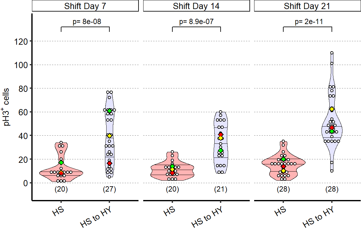
4.1.4 Figure 4D
Shifting between diets impacts pH3+ cell number in shrinkage (HY to HS) experiments. Statistical comparisons are vs pre-shift measurement.
Length_shrinkage_PH3 =
  d[["4C', 4S1D'"]]%>%
  mutate_at(vars(ends_with(".L")),~./1000)%>%
  mutate_at(vars(!starts_with("Total")),as.factor)%>%
  dplyr::rename(Total_Length_mm=Total.L,
         PH3_positive_cell=Total.PH3,
         Day_of_treatment=Day)%>%
  as.data.frame()%>%
  mutate(Dday=fct_relevel(Dday,"Shift Day 7","Shift Day 14","Shift Day 21"))

Sample_size=
  Length_shrinkage_PH3%>%
  group_by(Diet,Dday)%>%
  summarise(Sample_size=n())

###Stats
###Day 7
mod.gen = fitme(log(PH3_positive_cell) ~  Diet + (1 | Repeat),data = subset(Length_shrinkage_PH3,Dday=="Shift Day 7"))
shapiro.test(residuals(mod.gen))
    Shapiro-Wilk normality test

data:  residuals(mod.gen)
W = 0.96318, p-value = 0.1917bptest(log(PH3_positive_cell) ~ Diet + (1 / Repeat),data = subset(Length_shrinkage_PH3,Dday=="Shift Day 7"))
    studentized Breusch-Pagan test

data:  log(PH3_positive_cell) ~ Diet + (1/Repeat)
BP = 1.9935, df = 1, p-value = 0.158
mod.gen1 = fitme(log(PH3_positive_cell) ~ 1 + (1 | Repeat),data = subset(Length_shrinkage_PH3,Dday=="Shift Day 7"))
test = anova(mod.gen, mod.gen1)
Chi2_LRT_shrinkage = 2*(mod.gen$APHLs[["p_v"]]-mod.gen1$APHLs[["p_v"]])
tab_stat = data.frame(Comparison = as.character(paste("HS Day 7 vs HS to HY Day 14")),
Variable = as.character(paste("Shift Day 7")),
Rep = nlevels(Length_shrinkage_PH3$Repeat),
chi2_LR = round(as.numeric(test$basicLRT$chi2_LR), digits = 2),
intercept = format(mod.gen$fixef[1],digits=3),
estimate = format(mod.gen$fixef[2],digits=3),
df = as.numeric(test$basicLRT$df),
Pvalue = as.numeric(format(pchisq(Chi2_LRT_shrinkage,df=1,lower.tail = F),digits=1,scientific=F)))
tab_stat_7=tab_stat
#Day 14
mod.gen = fitme(log(PH3_positive_cell) ~ Diet + (1 | Repeat),data = subset(Length_shrinkage_PH3,Dday=="Shift Day 14"))
shapiro.test(residuals(mod.gen))
    Shapiro-Wilk normality test

data:  residuals(mod.gen)
W = 0.88271, p-value = 0.0008579bptest(log(PH3_positive_cell) ~ Diet + (1 / Repeat),data = subset(Length_shrinkage_PH3,Dday=="Shift Day 14"))
    studentized Breusch-Pagan test

data:  log(PH3_positive_cell) ~ Diet + (1/Repeat)
BP = 0.31605, df = 1, p-value = 0.574
mod.gen1 = fitme(log(PH3_positive_cell) ~ 1 + (1 | Repeat),data = subset(Length_shrinkage_PH3,Dday=="Shift Day 14"))
test = anova(mod.gen, mod.gen1)
Chi2_LRT_shrinkage = 2*(mod.gen$APHLs[["p_v"]]-mod.gen1$APHLs[["p_v"]])
tab_stat = data.frame(Comparison = as.character(paste("HS Day 14 vs HS to HY Day 21")),
Variable = as.character(paste("Shift Day 14")),
Rep = nlevels(Length_shrinkage_PH3$Repeat),
chi2_LR = round(as.numeric(test$basicLRT$chi2_LR), digits = 2),
intercept = format(mod.gen$fixef[1],digits=3),
estimate = format(mod.gen$fixef[2],digits=3),
df = as.numeric(test$basicLRT$df),
Pvalue = as.numeric(format(pchisq(Chi2_LRT_shrinkage,df=1,lower.tail = F),digits=1)))
tab_stat_14=tab_stat
#Day 21
mod.gen = fitme(log(PH3_positive_cell) ~ Diet + (1 | Repeat),data = subset(Length_shrinkage_PH3,Dday=="Shift Day 21"))
shapiro.test(residuals(mod.gen))
    Shapiro-Wilk normality test

data:  residuals(mod.gen)
W = 0.97516, p-value = 0.3966bptest(log(PH3_positive_cell) ~ Diet + (1 / Repeat),data = subset(Length_shrinkage_PH3,Dday=="Shift Day 21"))
    studentized Breusch-Pagan test

data:  log(PH3_positive_cell) ~ Diet + (1/Repeat)
BP = 0.66778, df = 1, p-value = 0.4138
mod.gen1 = fitme(log(PH3_positive_cell) ~ 1 + (1 | Repeat),data = subset(Length_shrinkage_PH3,Dday=="Shift Day 21"))
test = anova(mod.gen, mod.gen1)
Chi2_LRT_shrinkage = 2*(mod.gen$APHLs[["p_v"]]-mod.gen1$APHLs[["p_v"]])
tab_stat = data.frame(Comparison = as.character(paste("HS Day 21 vs HS to HY Day 28")),
Variable = as.character(paste("Shift Day 21")),
Rep = nlevels(Length_shrinkage_PH3$Repeat),
chi2_LR = round(as.numeric(test$basicLRT$chi2_LR), digits = 2),
intercept = format(mod.gen$fixef[1],digits=3),
estimate = format(mod.gen$fixef[2],digits=3),
df = as.numeric(test$basicLRT$df),
Pvalue = as.numeric(format(pchisq(Chi2_LRT_shrinkage,df=1,lower.tail = F),digits=2)))
tab_stat_21 = tab_stat
tab_stat=rbind(tab_stat_7,tab_stat_14,tab_stat_21)
tab_stat$sig = ifelse(tab_stat$Pvalue < 0.05 & tab_stat$Pvalue > 0.01, "*",
ifelse(tab_stat$Pvalue < 0.01 & tab_stat$Pvalue > 0.001, "**",
ifelse(tab_stat$Pvalue < 0.001, "***", "")))
tab_stat%>%
kable(col.names = c("Comparison", "Variable", "Replicates", "Chi2","Intercept","Estimate","df" ,"p-value","Signif."),row.names = FALSE) %>% add_header_above(c("log(PH3_positive_cell) ~ Diet + (1 | Repeat)" = 9))%>%
kable_styling(bootstrap_options = c("striped", "hover", "condensed"), full_width = F)| Comparison | Variable | Replicates | Chi2 | Intercept | Estimate | df | p-value | Signif. |
|---|---|---|---|---|---|---|---|---|
| HS Day 7 vs HS to HY Day 14 | Shift Day 7 | 3 | 1.93 | 3.56 | -0.25 | 1 | 2.0e-01 | |
| HS Day 14 vs HS to HY Day 21 | Shift Day 14 | 3 | 13.65 | 3.98 | -0.74 | 1 | 2.0e-04 | *** |
| HS Day 21 vs HS to HY Day 28 | Shift Day 21 | 3 | 20.21 | 4.18 | -0.59 | 1 | 6.9e-06 | *** |
tab_stat=
  tab_stat %>%
  dplyr::rename(Dday=Variable)%>%
  as.data.frame()%>%
  mutate(Dday=fct_relevel(Dday,"Shift Day 7","Shift Day 14","Shift Day 21"))

### Plot
Limits = c("HY","HYtoHS")
z = max(Length_shrinkage_PH3$PH3_positive_cell, na.rm = TRUE)

Plot_Fig4D=
  ggplot(Length_shrinkage_PH3, aes(x = Diet, y = PH3_positive_cell))+
  geom_violin(aes(fill = Diet), draw_quantiles = c(0.25, 0.5, 0.75), colour = "black", size = 0.2,adjust = 0.8) +
  geom_dotplot( colour = "black", fill = "white", binaxis = "y", stackdir = "center", binwidth = z/40) +
  facet_grid(. ~ Dday)+
  geom_text(data = Sample_size, mapping = aes(x = Diet, y = -5, label = paste("(",Sample_size,")",sep="")),size=3)+
      geom_signif(data = tab_stat, aes(xmin = 1, xmax = 2, annotations = formatC(paste("p=",Pvalue), digits = 2), y_position = 132,), textsize = 3, vjust = -0.2, manual = TRUE)+

  scale_fill_manual(limits=c("HY","HYtoHS"),
                    values=cbbHY_HYtoHS)+
  scale_x_discrete("",
                   limits=Limits,
                   labels=c("HY","HY to HS"))+
  scale_y_continuous(expression(paste("pH3" ^ "+", " cells")),
                     limits=c(-8,136),
                     breaks=seq(0,120,by=20))+
  stat_summary(fun = mean, geom = "point", size = 3, shape = 18, colour = "black", aes(group = Repeat)) +
                     stat_summary(fun = mean, geom = "point", size = 2, shape = 18, aes(group = Repeat, colour = Repeat)) +
                     scale_color_manual(values = palette_mean) +
  theme(panel.grid.major.y = element_line(colour = grey(0.45), linetype = "dashed", size = 0.2),
        panel.background = element_blank(),
        axis.title.x = element_text(size=Smallfont,colour="black"),
        axis.title.y = element_text(size=Smallfont,colour="black"),
        axis.line.x = element_line(colour="black",size=0.75),
        axis.line.y = element_line(colour="black",size=0.75),
        axis.ticks.x = element_line(size = 0.75),
        axis.ticks.y = element_line(size = 0.75),
        axis.text.x = element_text(size=Smallfont,colour="black",angle=30,hjust=1),
        axis.text.y = element_text(size=Smallfont,colour="black"),
        plot.margin = unit(Margin, "cm"),
        legend.direction = "vertical",
        legend.box = "horizontal",
        legend.position = "none",
        legend.key.height = unit(0.4, "cm"),
        legend.key.width= unit(0.6, "cm"),
        legend.title = element_text(face="italic",size=Smallfont),
        legend.key = element_rect(colour = 'white', fill = "white", linetype='dashed'),
        legend.text = element_text(size=SuperSmallfont),
        legend.background = element_rect(fill=NA),
        strip.text.x = element_text(size = Smallfont, colour = "black", margin = margin(t = 2, r = 0, b = 2, l = 0)),
        strip.text.y = element_text(size = Smallfont, colour = "black", margin = margin(t = 2, r = 0, b = 2, l = 0)),
        strip.background = element_rect(fill=NA, colour="black"),
        strip.placement="outside")

Plot_Fig4D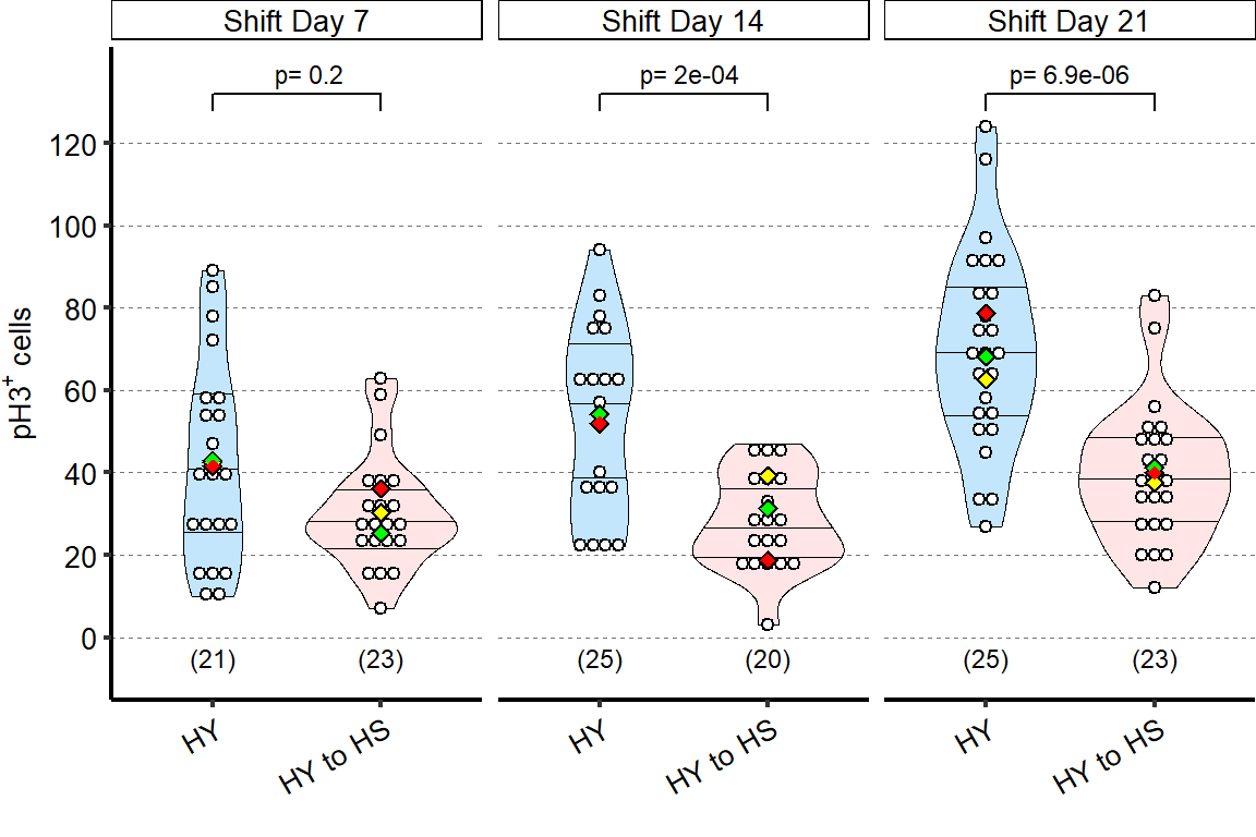
4.1.5 Figure 4E-F
Clonal assay with EsgF/O system illustrates increased number of marked cells on HY (F) vs HS (E) diets 5 days post-eclosion in region 4 of the midgut. GFP, in green, marks all cells made since the EsgF/O system was activated. Complete graphical annotation can be found in manuscript figures


4.1.6 Figure 4G-H-I-J
Cell loss assay enables analysis of the impact of diet composition on replacement ratio and rate. Description of experimental design is found in materials and methods and illustrated in figure 4–figure supplement 1H. In brief, this assay allows us to mark ECs and EBs at the start of the experiment and to count their numbers 14 days after shifting dietary conditions recapitulating growth and shrinkage of the midgut, thus estimating cell gain and cell loss in these conditions. Representative pictures for the cell loss assay in growing conditions (G, H, top row) and shrinkage conditions (I, J, bottom row). Complete graphical annotation can be found in manuscript figures
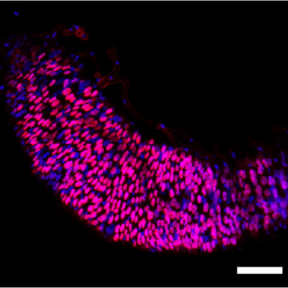
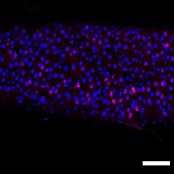
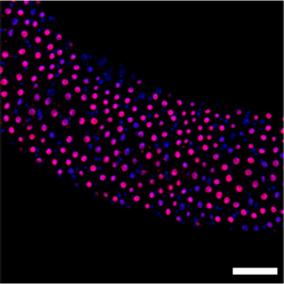

4.1.7 Figure 4K
In red 5966GS> His-RFP, marking EB and EC. Number of ECs in the posterior midgut, both marked (Red, old ECs) and unmarked (Blue, new ECs) by RFP, error bars are SE from 3 repeats.
tab_prop_cell_RFP =
  d[["4K"]]%>%
  mutate_if(is.character,as.factor)%>%
  mutate_if(is.integer,as.factor)%>%
  mutate(Post.Dapi.Number = (Post.Dapi.Number)*2)%>%
  mutate(Post.RFP.Number = (Post.RFP.Number)*2)%>%
  mutate(Post.NonRFP.Number = (Post.Dapi.Number - Post.RFP.Number))%>%
  group_by(Day, Diet, Diet1, Experiment)%>%
  summarise(mean_RFP_positive=mean(Post.RFP.Number,na.rm=T),
            se_RFP_positive=se(Post.RFP.Number),
            mean_RFP_negative=mean(Post.NonRFP.Number,na.rm=T),
            se_RFP_negative=se(Post.NonRFP.Number))%>%
  mutate(group=paste(Diet1,Experiment,sep="_"))%>%
  as.data.frame()

attach(tab_prop_cell_RFP)
for (i in 1:length(Experiment)){
    tab_prop_cell_RFP$se_proportionGraphPlus_pos[i] = mean_RFP_positive[i]+se_RFP_positive[i]
    tab_prop_cell_RFP$se_proportionGraphMinus_pos[i] = mean_RFP_positive[i]-se_RFP_positive[i]
    tab_prop_cell_RFP$se_proportionGraphPlus_neg[i] = mean_RFP_positive[i]+mean_RFP_negative[i]+se_RFP_negative[i]
    tab_prop_cell_RFP$se_proportionGraphMinus_neg[i] = mean_RFP_positive[i]+mean_RFP_negative[i]-se_RFP_negative[i]
}

tmp1 = tab_prop_cell_RFP[,c("Day", "Diet", "Diet1", "Experiment","mean_RFP_positive", "se_RFP_positive","se_proportionGraphPlus_pos", "se_proportionGraphMinus_pos")]
tmp1$RFP="Positive"
tmp1=dplyr::rename(tmp1,mean_RFP = mean_RFP_positive,
            se_RFP = se_RFP_positive,
            se_proportionGraphPlus =se_proportionGraphPlus_pos,
            se_proportionGraphMinus= se_proportionGraphMinus_pos)

tmp2 = tab_prop_cell_RFP[,c("Day", "Diet", "Diet1", "Experiment","mean_RFP_negative", "se_RFP_negative", "se_proportionGraphMinus_neg" ,"se_proportionGraphPlus_neg")]
tmp2$RFP="Negative"
tmp2=dplyr::rename(tmp2,mean_RFP = mean_RFP_negative,
            se_RFP = se_RFP_negative,
            se_proportionGraphPlus =se_proportionGraphPlus_neg,
            se_proportionGraphMinus= se_proportionGraphMinus_neg)

tab_prop_cell_RFP = rbind(tmp1,tmp2)
tab_prop_cell_RFP =
  tab_prop_cell_RFP%>%
  mutate_if(is.numeric,round,0)%>%
  mutate_if(is.character,as.factor)

#tab_prop_cell_RFP$Experiment = as.factor(ifelse(tab_prop_cell_RFP$Day=="0" & tab_prop_cell_RFP$Diet1=="HS","HS",
                                      #ifelse(tab_prop_cell_RFP$Day=="0" & tab_prop_cell_RFP$Diet1=="HY","HY",
                                            # as.character(tab_prop_cell_RFP$Experiment))))

#tab_prop_cell_RFP=
  #tab_prop_cell_RFP%>%
  #as.data.frame()%>%
  #mutate(Diet1=fct_relevel(Diet1,"HS", "HStoHS" , "HStoHY", "HY", "HYtoHS", "HYtoHY"),
         #Experiment=fct_relevel(Experiment, "HS", "Growth", "HY", "Shrinkage"))

levels(tab_prop_cell_RFP$Diet1) <- c("HS", "HS to HS" , "HS to HY", "HY", "HY to HS", "HY to HY")

Sample_size=
    d[["4K"]]%>%
  mutate_if(is.character,as.factor)%>%
  mutate_if(is.integer,as.factor)%>%
  group_by(Diet1)%>%
  summarise(Sample_size=n())

Sample_size$Experiment = c("G", "G", "G", "S", "S", "S")

levels(Sample_size$Diet1) <- c("HS", "HS to HS" , "HS to HY", "HY", "HY to HS", "HY to HY")


Plot_Fig4K =
  ggplot(tab_prop_cell_RFP, aes(x=Diet1, y=mean_RFP))+
  geom_bar(stat="identity",aes(fill=RFP),color="black",width=.90)+
  geom_errorbar(aes(ymin= se_proportionGraphMinus, ymax= se_proportionGraphPlus),width=0.25)+
   geom_text(data = Sample_size, mapping = aes(x = Diet1, y = 200, label = paste("(",Sample_size,")",sep="")),size=3)+
  facet_wrap(.~Experiment,scales="free_x")+
  scale_fill_manual(name = "RFP labelling",
                    values=c("#3a5ecc","#cc0000"),
                    labels = c("Negative", "Positive"))+
  scale_y_continuous("Number of cells (mean \u00B1se)",
                     limits=c(0,5800),
                     breaks=seq(0,5000,by=500))+
  theme(
    panel.grid.major.y = element_line(colour = grey(0.45), linetype = "dashed", size = 0.2),
    panel.background = element_blank(),
    axis.title.x = element_blank(),
    axis.title.y = element_text(size=Smallfont,colour="black"),
    axis.line.x = element_line(colour="black",size=0.75),
    axis.line.y = element_line(colour="black",size=0.75),
    axis.ticks.x = element_line(size = 0.75),
    axis.ticks.y = element_line(size = 0.75),
    axis.text.x = element_text(size=Smallfont,colour="black",angle=30,hjust=1),
    axis.text.y = element_text(size=Smallfont,colour="black"),
    plot.margin = unit(Margin, "cm"),
    legend.direction = "vertical",
    legend.box = "horizontal",
    legend.position = c(0.2,0.87),
    legend.key.height = unit(0.4, "cm"),
    legend.key.width= unit(0.6, "cm"),
    legend.title = element_text(face="italic",size=Smallfont),
    legend.key = element_rect(colour = 'white', fill = "white", linetype='dashed'),
    legend.text = element_text(size=Smallfont),
    legend.background = element_rect(fill=NA),
    strip.text = element_blank())
    #strip.background = element_rect(fill=NA, colour="black"),
    #strip.placement="outside")

Plot_Fig4K
4.1.8 Figure 4L
Data shown as rate relative to experiment start (cell /initial EC/ day). Number on bar in red is ratio of EC gained/EC lost (see materials and methods for formula).
tab_relative_cell_rate =
  d[["4L, 4S2D"]]%>%
  select(-starts_with("X"))%>%
  drop_na()%>%
  mutate_if(is.character,as.factor)%>%
  group_by(Diet1, Experiment, Experiment2, GL)%>%
  summarise(mean_RelativeRate=mean(RelativeRate,na.rm=T),
            se_RelativeRate=se(RelativeRate))%>%
            mutate(group=paste(Diet1,Experiment,sep="_"))%>%
  as.data.frame()


tab_relative_cell_rate_ratio =
  tab_relative_cell_rate%>%
  group_by(Diet1,Experiment2)%>%
  summarize(Ratio = round(mean_RelativeRate[GL == "Gain"] / (-mean_RelativeRate[GL == "Loss"]),2))%>%
  mutate(GL="Loss")

levels(tab_relative_cell_rate$Diet1) <- c("HS to HS" , "HS to HY", "HY to HS", "HY to HY")
levels(tab_relative_cell_rate_ratio$Diet1) <- c("HS to HS" , "HS to HY", "HY to HS", "HY to HY")


Plot_Fig4L =
  ggplot(tab_relative_cell_rate, aes(x = Diet1, y = mean_RelativeRate, fill = GL))+
  geom_bar(stat="identity",aes(fill=GL),color="black",width=.90)+
  geom_hline(yintercept = 0)+
  geom_text(data=tab_relative_cell_rate_ratio,mapping=aes(x=Diet1,y=-0.01,label=Ratio), color = "red")+
  facet_grid(.~Experiment2,scales="free_x")+

  scale_fill_manual(name = "Enterocyte",
                    values=c("palegreen", "moccasin"),
                    labels = c("Gain", "Loss"))+
  scale_y_continuous("Cell rate (cell/ initialEC/ day)",
                     limits=c(-0.11,0.11),
                     breaks=seq(-0.2,0.2,by=0.05))+
  theme(
    panel.grid.major.y = element_line(colour = grey(0.45), linetype = "dashed", size = 0.2),
    panel.background = element_blank(),
    axis.title.x = element_blank(),
    axis.title.y = element_text(size=Smallfont,colour="black"),
    axis.line.x = element_line(colour="black",size=0.75),
    axis.line.y = element_line(colour="black",size=0.75),
    axis.ticks.x = element_line(size = 0.75),
    axis.ticks.y = element_line(size = 0.75),
    axis.text.x = element_text(size=Smallfont,colour="black",angle=30,hjust=1),
    axis.text.y = element_text(size=Smallfont,colour="black"),
    plot.margin = unit(Margin, "cm"),
    legend.direction = "vertical",
    legend.box = "horizontal",
    legend.position = c(0.18,0.83),
    legend.key.height = unit(0.4, "cm"),
    legend.key.width= unit(0.6, "cm"),
    legend.title = element_text(face="italic",size=Smallfont),
    legend.key = element_rect(colour = 'white', fill = "white", linetype='dashed'),
    legend.text = element_text(size=Smallfont),
    legend.background = element_rect(fill=NA),
    strip.text.x = element_text(size = Smallfont, colour = "black", margin = margin(t = 2, r = 0, b = 2, l = 0)),
    strip.text.y = element_text(size = Smallfont, colour = "black", margin = margin(t = 2, r = 0, b = 2, l = 0)),
    strip.background = element_rect(fill=NA, colour="black"),
    strip.placement="outside")


Plot_Fig4L
##Export Figure 4
4.2 Figure 4 - supplementary 1
4.2.1 Figure 4S1A
Midgut length increases progressively on HY, but not on HS. Statistics compare HS vs HY for each day, *** = p<0.01.
Length_dayseclosion =
  d[["4 - S1A"]]%>%
  select(-starts_with("X"))%>%
  mutate_at(vars(starts_with("Total")),~./1000)%>%
  mutate_if(is.character,as.factor)%>%
  mutate_if(is.integer,as.factor)%>%
  dplyr::rename(Total_Length_mm=Total.Length)%>%
  mutate(group=paste(TreatCol,Day,sep="_"))

Sample_size=
  Length_dayseclosion%>%
  group_by(Day,TreatCol)%>%
  summarise(Sample_size=n())%>%
  dplyr::rename(Diet=TreatCol)

#Stats4S1A
###Stats

#Day 1
tmp = subset(Length_dayseclosion, Day == "1") %>%
    mutate(Day = as.factor(Day))

mod.gen = fitme(log(Total_Length_mm) ~ Diet + (1 | Repeat), data = tmp)
shapiro.test(residuals(mod.gen))
    Shapiro-Wilk normality test

data:  residuals(mod.gen)
W = 0.97708, p-value = 0.614bptest(log(Total_Length_mm) ~ Diet + (1 / Repeat), data = tmp)
    studentized Breusch-Pagan test

data:  log(Total_Length_mm) ~ Diet + (1/Repeat)
BP = 0.1261, df = 1, p-value = 0.7225
mod.gen1 = fitme(log(Total_Length_mm) ~ 1 + (1 | Repeat), data = tmp)
test = anova(mod.gen, mod.gen1)
Chi2_LRT_growth = 2 * (mod.gen$APHLs[["p_v"]] - mod.gen1$APHLs[["p_v"]])
tab_stat = data.frame(Variable = as.character("1"),
Rep = nlevels(tmp$Repeat),
chi2_LR = round(as.numeric(test$basicLRT$chi2_LR), digits = 2),
intercept = format(mod.gen$fixef[1],digits=3),
estimate = format(mod.gen$fixef[2],digits=3),
df = as.numeric(test$basicLRT$df),
Pvalue = as.numeric(format(pchisq(Chi2_LRT_growth,df=1,lower.tail = F),digits=2)))
tab_stat_day_1 = tab_stat
#Day 2
tmp = subset(Length_dayseclosion, Day == "2") %>%
mutate(Day = as.factor(Day))
mod.gen = fitme(log(Total_Length_mm) ~ Diet + (1 | Repeat), data = tmp)
shapiro.test(residuals(mod.gen))
    Shapiro-Wilk normality test

data:  residuals(mod.gen)
W = 0.99417, p-value = 0.9992bptest(log(Total_Length_mm) ~ Diet + (1 / Repeat), data = tmp)
    studentized Breusch-Pagan test

data:  log(Total_Length_mm) ~ Diet + (1/Repeat)
BP = 1.0007, df = 1, p-value = 0.3171
mod.gen1 = fitme(log(Total_Length_mm) ~ 1 + (1 | Repeat), data = tmp)
test = anova(mod.gen, mod.gen1)
Chi2_LRT_growth = 2 * (mod.gen$APHLs[["p_v"]] - mod.gen1$APHLs[["p_v"]])
tab_stat = data.frame(Variable = as.character("2"),
Rep = nlevels(tmp$Repeat),
chi2_LR = round(as.numeric(test$basicLRT$chi2_LR), digits = 2),
intercept = format(mod.gen$fixef[1],digits=3),
estimate = format(mod.gen$fixef[2],digits=3),
df = as.numeric(test$basicLRT$df),
Pvalue = as.numeric(format(pchisq(Chi2_LRT_growth,df=1,lower.tail = F),digits=2)))
tab_stat_day_2 = tab_stat
#Day 3
tmp = subset(Length_dayseclosion, Day == "3") %>%
mutate(Day = as.factor(Day))
mod.gen = fitme(log(Total_Length_mm) ~ Diet + (1 | Repeat), data = tmp)
shapiro.test(residuals(mod.gen))
    Shapiro-Wilk normality test

data:  residuals(mod.gen)
W = 0.98604, p-value = 0.8874bptest(log(Total_Length_mm) ~ Diet + (1 / Repeat), data = tmp)
    studentized Breusch-Pagan test

data:  log(Total_Length_mm) ~ Diet + (1/Repeat)
BP = 4.4343, df = 1, p-value = 0.03522
mod.gen1 = fitme(log(Total_Length_mm) ~ 1 + (1 | Repeat), data = tmp)
test = anova(mod.gen, mod.gen1)
Chi2_LRT_growth = 2 * (mod.gen$APHLs[["p_v"]] - mod.gen1$APHLs[["p_v"]])
tab_stat = data.frame(Variable = as.character("3"),
Rep = nlevels(tmp$Repeat),
chi2_LR = round(as.numeric(test$basicLRT$chi2_LR), digits = 2),
intercept = format(mod.gen$fixef[1],digits=3),
estimate = format(mod.gen$fixef[2],digits=3),
df = as.numeric(test$basicLRT$df),
Pvalue = as.numeric(format(pchisq(Chi2_LRT_growth,df=1,lower.tail = F),digits=2)))
tab_stat_day_3 = tab_stat
#Day 4
tmp = subset(Length_dayseclosion, Day == "4") %>%
mutate(Day = as.factor(Day))
mod.gen = fitme(log(Total_Length_mm) ~ Diet + (1 | Repeat), data = tmp)
shapiro.test(residuals(mod.gen))
    Shapiro-Wilk normality test

data:  residuals(mod.gen)
W = 0.98212, p-value = 0.7675bptest(log(Total_Length_mm) ~ Diet + (1 / Repeat), data = tmp)
    studentized Breusch-Pagan test

data:  log(Total_Length_mm) ~ Diet + (1/Repeat)
BP = 2.4272, df = 1, p-value = 0.1192
mod.gen1 = fitme(log(Total_Length_mm) ~ 1 + (1 | Repeat), data = tmp)
test = anova(mod.gen, mod.gen1)
Chi2_LRT_growth = 2 * (mod.gen$APHLs[["p_v"]] - mod.gen1$APHLs[["p_v"]])
tab_stat = data.frame(Variable = as.character(paste("4")),
Rep = nlevels(tmp$Repeat),
chi2_LR = round(as.numeric(test$basicLRT$chi2_LR), digits = 2),
intercept = format(mod.gen$fixef[1],digits=3),
estimate = format(mod.gen$fixef[2],digits=3),
df = as.numeric(test$basicLRT$df),
Pvalue = as.numeric(format(pchisq(Chi2_LRT_growth,df=1,lower.tail = F),digits=2)))
tab_stat_day_4 = tab_stat
#Day 5
tmp = subset(Length_dayseclosion, Day == "5") %>%
mutate(Day = as.factor(Day))
mod.gen = fitme(log(Total_Length_mm) ~ Diet + (1 | Repeat), data = tmp)
shapiro.test(residuals(mod.gen))
    Shapiro-Wilk normality test

data:  residuals(mod.gen)
W = 0.98337, p-value = 0.8115bptest(log(Total_Length_mm) ~ Diet + (1 / Repeat), data = tmp)
    studentized Breusch-Pagan test

data:  log(Total_Length_mm) ~ Diet + (1/Repeat)
BP = 0.17809, df = 1, p-value = 0.673
mod.gen1 = fitme(log(Total_Length_mm) ~ 1 + (1 | Repeat), data = tmp)
test = anova(mod.gen, mod.gen1)
Chi2_LRT_growth = 2 * (mod.gen$APHLs[["p_v"]] - mod.gen1$APHLs[["p_v"]])
tab_stat = data.frame(Variable = as.character("5"),
Rep = nlevels(tmp$Repeat),
chi2_LR = round(as.numeric(test$basicLRT$chi2_LR), digits = 2),
intercept = format(mod.gen$fixef[1],digits=3),
estimate = format(mod.gen$fixef[2],digits=3),
df = as.numeric(test$basicLRT$df),
Pvalue = as.numeric(format(pchisq(Chi2_LRT_growth,df=1,lower.tail = F),digits=2)))
tab_stat_day_5 = tab_stat
tab_stat = rbind(tab_stat_day_1, tab_stat_day_2, tab_stat_day_3, tab_stat_day_4, tab_stat_day_5)
tab_stat$padj = p.adjust(tab_stat$Pvalue, method = "BH")
tab_stat$sig = ifelse(tab_stat$padj < 0.05 & tab_stat$padj > 0.01, "*",
ifelse(tab_stat$padj < 0.01 & tab_stat$padj > 0.001, "**",
ifelse(tab_stat$padj < 0.001, "***", "")))
tab_stat%>%
kable(col.names = c("Comparisons diet within days", "Replicates", "Chi2","Intercept","Estimate","df" ,"p-value","p-value adjusted","Signif."),row.names = FALSE) %>%
add_header_above(c("log(Total_Length_mm) ~ Diet + (1 | Repeat)" = 9))%>%
kable_styling(bootstrap_options = c("striped", "hover", "condensed"), full_width = F)| Comparisons diet within days | Replicates | Chi2 | Intercept | Estimate | df | p-value | p-value adjusted | Signif. |
|---|---|---|---|---|---|---|---|---|
| 1 | 3 | 12.43 | 1.58 | 0.095 | 1 | 4.2e-04 | 4.20e-04 | *** |
| 2 | 3 | 23.56 | 1.59 | 0.167 | 1 | 1.2e-06 | 2.00e-06 | *** |
| 3 | 3 | 13.67 | 1.64 | 0.122 | 1 | 2.2e-04 | 2.75e-04 | *** |
| 4 | 3 | 45.37 | 1.52 | 0.271 | 1 | 0.0e+00 | 0.00e+00 | *** |
| 5 | 3 | 30.29 | 1.57 | 0.244 | 1 | 0.0e+00 | 1.00e-07 | *** |
tab_stat =
    tab_stat %>%
    dplyr::rename(Day = Variable) %>%
    mutate(Day = as.factor(Day))
tab_stat$Diet = "HY"

letter_position = aggregate(data = Length_dayseclosion, Total_Length_mm ~ Day, max)

tab_stat1 = left_join(tab_stat, letter_position)

#Stats vs eclosion for HS

Length_dayseclosionHS = subset(Length_dayseclosion, Diet == "0" | Diet == "HS")
#Day 1
tmp = subset(Length_dayseclosionHS, Day == "0" | Day == "1") %>%
    mutate(Day = as.factor(Day))

mod.gen = fitme(log(Total_Length_mm) ~ Day + (1 | Repeat), data = tmp)
shapiro.test(residuals(mod.gen))
    Shapiro-Wilk normality test

data:  residuals(mod.gen)
W = 0.99072, p-value = 0.9926bptest(log(Total_Length_mm) ~ Day + (1 / Repeat), data = tmp)
    studentized Breusch-Pagan test

data:  log(Total_Length_mm) ~ Day + (1/Repeat)
BP = 1.1212, df = 1, p-value = 0.2897
mod.gen1 = fitme(log(Total_Length_mm) ~ 1 + (1 | Repeat), data = tmp)
test = anova(mod.gen, mod.gen1)
Chi2_LRT_growth = 2 * (mod.gen$APHLs[["p_v"]] - mod.gen1$APHLs[["p_v"]])
tab_stat = data.frame(Variable = as.character(paste("1")),
Rep = nlevels(tmp$Repeat),
chi2_LR = round(as.numeric(test$basicLRT$chi2_LR), digits = 2),
intercept = format(mod.gen$fixef[1],digits=3),
estimate = format(mod.gen$fixef[2],digits=3),
df = as.numeric(test$basicLRT$df),
Pvalue = as.numeric(format(pchisq(Chi2_LRT_growth,df=1,lower.tail = F),digits=2)))
tab_stat_day_0vs1 = tab_stat
#Day 2
tmp = subset(Length_dayseclosionHS, Day == "0" | Day == "2") %>%
mutate(Day = as.factor(Day))
mod.gen = fitme(log(Total_Length_mm) ~ Day + (1 | Repeat), data = tmp)
shapiro.test(residuals(mod.gen))
    Shapiro-Wilk normality test

data:  residuals(mod.gen)
W = 0.96616, p-value = 0.4006bptest(log(Total_Length_mm) ~ Day + (1 / Repeat), data = tmp)
    studentized Breusch-Pagan test

data:  log(Total_Length_mm) ~ Day + (1/Repeat)
BP = 0.15716, df = 1, p-value = 0.6918
mod.gen1 = fitme(log(Total_Length_mm) ~ 1 + (1 | Repeat), data = tmp)
test = anova(mod.gen, mod.gen1)
Chi2_LRT_growth = 2 * (mod.gen$APHLs[["p_v"]] - mod.gen1$APHLs[["p_v"]])
tab_stat = data.frame(Variable = as.character(paste("2")),
Rep = nlevels(tmp$Repeat),
chi2_LR = round(as.numeric(test$basicLRT$chi2_LR), digits = 2),
intercept = format(mod.gen$fixef[1],digits=3),
estimate = format(mod.gen$fixef[2],digits=3),
df = as.numeric(test$basicLRT$df),
Pvalue = as.numeric(format(pchisq(Chi2_LRT_growth,df=1,lower.tail = F),digits=2)))
tab_stat_day_0vs2 = tab_stat
#Day 3
tmp = subset(Length_dayseclosionHS, Day == "0" | Day == "3") %>%
mutate(Day = as.factor(Day))
mod.gen = fitme(log(Total_Length_mm) ~ Day + (1 | Repeat), data = tmp)
shapiro.test(residuals(mod.gen))
Shapiro-Wilk normality test
data: residuals(mod.gen)
W = 0.98717, p-value = 0.9438bptest(log(Total_Length_mm) ~ Day + (1 / Repeat), data = tmp)
studentized Breusch-Pagan test
data: log(Total_Length_mm) ~ Day + (1/Repeat)
BP = 0.11255, df = 1, p-value = 0.7373mod.gen1 = fitme(log(Total_Length_mm) ~ 1 + (1 | Repeat), data = tmp)
test = anova(mod.gen, mod.gen1)
Chi2_LRT_growth = 2 * (mod.gen$APHLs[["p_v"]] - mod.gen1$APHLs[["p_v"]])
tab_stat = data.frame(Variable = as.character(paste("3")),
Rep = nlevels(tmp$Repeat),
chi2_LR = round(as.numeric(test$basicLRT$chi2_LR), digits = 2),
intercept = format(mod.gen$fixef[1],digits=3),
estimate = format(mod.gen$fixef[2],digits=3),
df = as.numeric(test$basicLRT$df),
Pvalue = as.numeric(format(pchisq(Chi2_LRT_growth,df=1,lower.tail = F),digits=2)))
tab_stat_day_0vs3 = tab_stat
#Day 4
tmp = subset(Length_dayseclosionHS, Day == "0" | Day == "4") %>%
mutate(Day = as.factor(Day))
mod.gen = fitme(log(Total_Length_mm) ~ Day + (1 | Repeat), data = tmp)
shapiro.test(residuals(mod.gen))
Shapiro-Wilk normality test
data: residuals(mod.gen)
W = 0.98443, p-value = 0.8899bptest(log(Total_Length_mm) ~ Day + (1 / Repeat), data = tmp)
studentized Breusch-Pagan test
data: log(Total_Length_mm) ~ Day + (1/Repeat)
BP = 2.049, df = 1, p-value = 0.1523mod.gen1 = fitme(log(Total_Length_mm) ~ 1 + (1 | Repeat), data = tmp)
test = anova(mod.gen, mod.gen1)
Chi2_LRT_growth = 2 * (mod.gen$APHLs[["p_v"]] - mod.gen1$APHLs[["p_v"]])
tab_stat = data.frame(Variable = as.character(paste("4")),
Rep = nlevels(tmp$Repeat),
chi2_LR = round(as.numeric(test$basicLRT$chi2_LR), digits = 2),
intercept = format(mod.gen$fixef[1],digits=3),
estimate = format(mod.gen$fixef[2],digits=3),
df = as.numeric(test$basicLRT$df),
Pvalue = as.numeric(format(pchisq(Chi2_LRT_growth,df=1,lower.tail = F),digits=2)))
tab_stat_day_0vs4 = tab_stat
#Day 5
tmp = subset(Length_dayseclosionHS, Day == "0" | Day == "5") %>%
mutate(Day = as.factor(Day))
mod.gen = fitme(log(Total_Length_mm) ~ Day + (1 | Repeat), data = tmp)
shapiro.test(residuals(mod.gen))
Shapiro-Wilk normality test
data: residuals(mod.gen)
W = 0.97527, p-value = 0.5856bptest(log(Total_Length_mm) ~ Day + (1 / Repeat), data = tmp)
studentized Breusch-Pagan test
data: log(Total_Length_mm) ~ Day + (1/Repeat)
BP = 0.010695, df = 1, p-value = 0.9176mod.gen1 = fitme(log(Total_Length_mm) ~ 1 + (1 | Repeat), data = tmp)
test = anova(mod.gen, mod.gen1)
Chi2_LRT_growth = 2 * (mod.gen$APHLs[["p_v"]] - mod.gen1$APHLs[["p_v"]])
tab_stat = data.frame(Variable = as.character(paste("5")),
Rep = nlevels(tmp$Repeat),
chi2_LR = round(as.numeric(test$basicLRT$chi2_LR), digits = 2),
intercept = format(mod.gen$fixef[1],digits=3),
estimate = format(mod.gen$fixef[2],digits=3),
df = as.numeric(test$basicLRT$df),
Pvalue = as.numeric(format(pchisq(Chi2_LRT_growth,df=1,lower.tail = F),digits=2)))
tab_stat_day_0vs5 = tab_stat
tab_statHSeclosion = rbind(tab_stat_day_0vs1, tab_stat_day_0vs2, tab_stat_day_0vs3, tab_stat_day_0vs4, tab_stat_day_0vs5)
tab_statHSeclosion$padj = p.adjust(tab_statHSeclosion$Pvalue, method = "BH")
tab_statHSeclosion$sig = ifelse(tab_statHSeclosion$padj > 0.05, "ns",
ifelse(tab_statHSeclosion$padj < 0.05 & tab_statHSeclosion$padj > 0.01, "*",
ifelse(tab_statHSeclosion$padj < 0.01 & tab_statHSeclosion$padj > 0.001, "**",
ifelse(tab_statHSeclosion$padj < 0.001, "***", ""))))
tab_statHSeclosion%>%
kable(col.names = c("Comparison to eclosion on HS", "Replicates", "Chi2","Intercept","Estimate","df" ,"p-value","p-value adjusted","Signif."),row.names = FALSE) %>%
add_header_above(c("log(Total_Length_mm) ~ Day + (1 | Repeat)" = 9))%>%
kable_styling(bootstrap_options = c("striped", "hover", "condensed"), full_width = F)| Comparison to eclosion on HS | Replicates | Chi2 | Intercept | Estimate | df | p-value | p-value adjusted | Signif. |
|---|---|---|---|---|---|---|---|---|
| 1 | 3 | 1.28 | 1.54 | 0.0399 | 1 | 0.260 | 0.4333333 | ns |
| 2 | 3 | 1.34 | 1.55 | 0.0447 | 1 | 0.250 | 0.4333333 | ns |
| 3 | 3 | 4.80 | 1.55 | 0.0868 | 1 | 0.028 | 0.1400000 | ns |
| 4 | 3 | 0.60 | 1.54 | -0.0244 | 1 | 0.440 | 0.4400000 | ns |
| 5 | 3 | 0.74 | 1.54 | 0.0319 | 1 | 0.390 | 0.4400000 | ns |
tab_statHSeclosion =
tab_statHSeclosion %>%
dplyr::rename(Day = Variable) %>%
mutate(Day = as.factor(Day))
tab_statHSeclosion$Diet = "HS"
letter_position = aggregate(data = Length_dayseclosion, Total_Length_mm ~ Day, max)
tab_statHSeclosion = left_join(tab_statHSeclosion, letter_position)
#Stats vs eclosion for HY
Length_dayseclosionHS = subset(Length_dayseclosion, Diet == "0" | Diet == "HY")
#Day 1
tmp = subset(Length_dayseclosionHS, Day == "0" | Day == "1") %>%
mutate(Day = as.factor(Day))
mod.gen = fitme(log(Total_Length_mm) ~ Day + (1 | Repeat), data = tmp)
shapiro.test(residuals(mod.gen))
Shapiro-Wilk normality test
data: residuals(mod.gen)
W = 0.96951, p-value = 0.4124bptest(log(Total_Length_mm) ~ Day + (1 / Repeat), data = tmp)
studentized Breusch-Pagan test
data: log(Total_Length_mm) ~ Day + (1/Repeat)
BP = 1.8328, df = 1, p-value = 0.1758mod.gen1 = fitme(log(Total_Length_mm) ~ 1 + (1 | Repeat), data = tmp)
test = anova(mod.gen, mod.gen1)
Chi2_LRT_growth = 2 * (mod.gen$APHLs[["p_v"]] - mod.gen1$APHLs[["p_v"]])
tab_stat = data.frame(Variable = as.character(paste("1")),
Rep = nlevels(tmp$Repeat),
chi2_LR = round(as.numeric(test$basicLRT$chi2_LR), digits = 2),
intercept = format(mod.gen$fixef[1],digits=3),
estimate = format(mod.gen$fixef[2],digits=3),
df = as.numeric(test$basicLRT$df),
Pvalue = as.numeric(format(pchisq(Chi2_LRT_growth,df=1,lower.tail = F),digits=2)))
tab_stat_day_0vs1 = tab_stat
#Day 2
tmp = subset(Length_dayseclosionHS, Day == "0" | Day == "2") %>%
mutate(Day = as.factor(Day))
mod.gen = fitme(log(Total_Length_mm) ~ Day + (1 | Repeat), data = tmp)
shapiro.test(residuals(mod.gen))
Shapiro-Wilk normality test
data: residuals(mod.gen)
W = 0.98822, p-value = 0.9615bptest(log(Total_Length_mm) ~ Day + (1 / Repeat), data = tmp)
studentized Breusch-Pagan test
data: log(Total_Length_mm) ~ Day + (1/Repeat)
BP = 1.6976, df = 1, p-value = 0.1926mod.gen1 = fitme(log(Total_Length_mm) ~ 1 + (1 | Repeat), data = tmp)
test = anova(mod.gen, mod.gen1)
Chi2_LRT_growth = 2 * (mod.gen$APHLs[["p_v"]] - mod.gen1$APHLs[["p_v"]])
tab_stat = data.frame(Variable = as.character(paste("2")),
Rep = nlevels(tmp$Repeat),
chi2_LR = round(as.numeric(test$basicLRT$chi2_LR), digits = 2),
intercept = format(mod.gen$fixef[1],digits=3),
estimate = format(mod.gen$fixef[2],digits=3),
df = as.numeric(test$basicLRT$df),
Pvalue = as.numeric(format(pchisq(Chi2_LRT_growth,df=1,lower.tail = F),digits=2)))
tab_stat_day_0vs2 = tab_stat
#Day 3
tmp = subset(Length_dayseclosionHS, Day == "0" | Day == "3") %>%
mutate(Day = as.factor(Day))
mod.gen = fitme(log(Total_Length_mm) ~ Day + (1 | Repeat), data = tmp)
shapiro.test(residuals(mod.gen))
Shapiro-Wilk normality test
data: residuals(mod.gen)
W = 0.98545, p-value = 0.9144bptest(log(Total_Length_mm) ~ Day + (1 / Repeat), data = tmp)
studentized Breusch-Pagan test
data: log(Total_Length_mm) ~ Day + (1/Repeat)
BP = 3.1177, df = 1, p-value = 0.07745mod.gen1 = fitme(log(Total_Length_mm) ~ 1 + (1 | Repeat), data = tmp)
test = anova(mod.gen, mod.gen1)
Chi2_LRT_growth = 2 * (mod.gen$APHLs[["p_v"]] - mod.gen1$APHLs[["p_v"]])
tab_stat = data.frame(Variable = as.character(paste("3")),
Rep = nlevels(tmp$Repeat),
chi2_LR = round(as.numeric(test$basicLRT$chi2_LR), digits = 2),
intercept = format(mod.gen$fixef[1],digits=3),
estimate = format(mod.gen$fixef[2],digits=3),
df = as.numeric(test$basicLRT$df),
Pvalue = as.numeric(format(pchisq(Chi2_LRT_growth,df=1,lower.tail = F),digits=2)))
tab_stat_day_0vs3 = tab_stat
#Day 4
tmp = subset(Length_dayseclosionHS, Day == "0" | Day == "4") %>%
mutate(Day = as.factor(Day))
mod.gen = fitme(log(Total_Length_mm) ~ Day + (1 | Repeat), data = tmp)
shapiro.test(residuals(mod.gen))
Shapiro-Wilk normality test
data: residuals(mod.gen)
W = 0.97795, p-value = 0.6915bptest(log(Total_Length_mm) ~ Day + (1 / Repeat), data = tmp)
studentized Breusch-Pagan test
data: log(Total_Length_mm) ~ Day + (1/Repeat)
BP = 0.026163, df = 1, p-value = 0.8715mod.gen1 = fitme(log(Total_Length_mm) ~ 1 + (1 | Repeat), data = tmp)
test = anova(mod.gen, mod.gen1)
Chi2_LRT_growth = 2 * (mod.gen$APHLs[["p_v"]] - mod.gen1$APHLs[["p_v"]])
tab_stat = data.frame(Variable = as.character(paste("4")),
Rep = nlevels(tmp$Repeat),
chi2_LR = round(as.numeric(test$basicLRT$chi2_LR), digits = 2),
intercept = format(mod.gen$fixef[1],digits=3),
estimate = format(mod.gen$fixef[2],digits=3),
df = as.numeric(test$basicLRT$df),
Pvalue = as.numeric(format(pchisq(Chi2_LRT_growth,df=1,lower.tail = F),digits=2)))
tab_stat_day_0vs4 = tab_stat
#Day 5
tmp = subset(Length_dayseclosionHS, Day == "0" | Day == "5") %>%
mutate(Day = as.factor(Day))
mod.gen = fitme(log(Total_Length_mm) ~ Day + (1 | Repeat), data = tmp)
shapiro.test(residuals(mod.gen))
Shapiro-Wilk normality test
data: residuals(mod.gen)
W = 0.98099, p-value = 0.8035bptest(log(Total_Length_mm) ~ Day + (1 / Repeat), data = tmp)
studentized Breusch-Pagan test
data: log(Total_Length_mm) ~ Day + (1/Repeat)
BP = 0.21338, df = 1, p-value = 0.6441mod.gen1 = fitme(log(Total_Length_mm) ~ 1 + (1 | Repeat), data = tmp)
test = anova(mod.gen, mod.gen1)
Chi2_LRT_growth = 2 * (mod.gen$APHLs[["p_v"]] - mod.gen1$APHLs[["p_v"]])
tab_stat = data.frame(Variable = as.character(paste("5")),
Rep = nlevels(tmp$Repeat),
chi2_LR = round(as.numeric(test$basicLRT$chi2_LR), digits = 2),
intercept = format(mod.gen$fixef[1],digits=3),
estimate = format(mod.gen$fixef[2],digits=3),
df = as.numeric(test$basicLRT$df),
Pvalue = as.numeric(format(pchisq(Chi2_LRT_growth,df=1,lower.tail = F),digits=2)))
tab_stat_day_0vs5 = tab_stat
tab_statHYeclosion = rbind(tab_stat_day_0vs1, tab_stat_day_0vs2, tab_stat_day_0vs3, tab_stat_day_0vs4, tab_stat_day_0vs5)
tab_statHYeclosion$padj = as.numeric(p.adjust(tab_statHYeclosion$Pvalue, method = "BH"))
tab_statHYeclosion$sig = ifelse(tab_statHYeclosion$padj > 0.05, "ns",
ifelse(tab_statHYeclosion$padj < 0.05 & tab_statHYeclosion$padj > 0.01, "*",
ifelse(tab_statHYeclosion$padj < 0.01 & tab_statHYeclosion$padj > 0.001, "**",
ifelse(tab_statHYeclosion$padj < 0.001, "***", ""))))
tab_statHYeclosion%>%
kable(col.names = c("Comparison to eclosion on HY", "Replicates", "Chi2","Intercept","Estimate","df" ,"p-value","p-value adjusted","Signif."),row.names = FALSE) %>%
add_header_above(c("log(Total_Length_mm) ~ Day + (1 | Repeat)" = 9))%>%
kable_styling(bootstrap_options = c("striped", "hover", "condensed"), full_width = F)| Comparison to eclosion on HY | Replicates | Chi2 | Intercept | Estimate | df | p-value | p-value adjusted | Signif. |
|---|---|---|---|---|---|---|---|---|
| 1 | 3 | 15.38 | 1.53 | 0.141 | 1 | 8.8e-05 | 8.8e-05 | *** |
| 2 | 3 | 28.64 | 1.55 | 0.209 | 1 | 1.0e-07 | 2.0e-07 | *** |
| 3 | 3 | 29.67 | 1.55 | 0.209 | 1 | 1.0e-07 | 2.0e-07 | *** |
| 4 | 3 | 27.96 | 1.55 | 0.24 | 1 | 1.0e-07 | 2.0e-07 | *** |
| 5 | 3 | 28.06 | 1.55 | 0.263 | 1 | 1.0e-07 | 2.0e-07 | *** |
tab_statHYeclosion =
tab_statHYeclosion %>%
dplyr::rename(Day = Variable) %>%
mutate(Day = as.factor(Day))
tab_statHYeclosion$Diet = "HY"
letter_position = aggregate(data = Length_dayseclosion, Total_Length_mm ~ Day, max)
tab_statHYeclosion = left_join(tab_statHYeclosion, letter_position)
### Plot
z = max(Length_dayseclosion$Total_Length_mm, na.rm = TRUE)
Plot_Fig4S1A=
ggplot(Length_dayseclosion, aes(x = Day, y = Total_Length_mm))+
geom_violin(aes(fill = Diet), draw_quantiles = c(0.25, 0.5, 0.75), colour = "black", size = 0.2,adjust = 0.8) +
geom_dotplot( colour = "black", fill = "white", binaxis = "y", stackdir = "center", binwidth = z/60) +
facet_grid(.~Diet,scales="free_x",space="free")+
geom_text(data = Sample_size, mapping = aes(x = Day, y = 2.3, label = paste("(",Sample_size,")",sep="")),size=3)+
geom_text(data = tab_stat1, mapping = aes(x =Day, y = 7.5, label = sig),size=3)+
geom_text(data = tab_statHSeclosion, mapping = aes(x =Day, y = 3.5, label = sig),size=3)+
geom_text(data = tab_statHYeclosion, mapping = aes(x =Day, y = 3.5, label = sig),size=3)+
scale_fill_manual(limits=c("0","HS","HY"),
values= c("#cfe7cf","#FFB4B4", "#C3E6FC"))+
scale_x_discrete("Days post eclosion")+
scale_y_continuous("Midgut length (mm)",
limits=c(2,8.2),
breaks=seq(2,8,by=1))+
stat_summary(fun = mean, geom = "point", size = 3, shape = 18, colour = "black", aes(group = Repeat)) +
stat_summary(fun = mean, geom = "point", size = 2, shape = 18, aes(group = Repeat, colour = Repeat)) +
scale_color_manual(values = palette_mean) +
theme(panel.grid.major.y = element_line(colour = grey(0.45), linetype = "dashed", size = 0.2),
panel.background = element_blank(),
axis.title.x = element_text(size=Smallfont,colour="black"),
axis.title.y = element_text(size=Smallfont,colour="black"),
axis.line.x = element_line(colour="black",size=0.75),
axis.line.y = element_line(colour="black",size=0.75),
axis.ticks.x = element_line(size = 0.75),
axis.ticks.y = element_line(size = 0.75),
axis.text.x = element_text(size=Smallfont,colour="black"),
axis.text.y = element_text(size=Smallfont,colour="black"),
plot.margin = unit(Margin, "cm"),
legend.direction = "vertical",
legend.box = "horizontal",
legend.position = "none",
legend.key.height = unit(0.4, "cm"),
legend.key.width= unit(0.6, "cm"),
legend.title = element_text(face="italic",size=Smallfont),
legend.key = element_rect(colour = 'white', fill = "white", linetype='dashed'),
legend.text = element_text(size=SuperSmallfont),
legend.background = element_rect(fill=NA),
strip.text.x = element_text(size = Smallfont, colour = "black", margin = margin(t = 2, r = 0, b = 2, l = 0)),
strip.text.y = element_text(size = Smallfont, colour = "black", margin = margin(t = 2, r = 0, b = 2, l = 0)),
strip.background = element_rect(fill=NA, colour="black"),
strip.placement="outside")
Plot_Fig4S1A
4.2.2 Figure 4S1B
Scheme for Figure 4 B, C, D and Figure 4 supplement 1C, D, E. At eclosion, flies were allocated to either HS or HY diet. 7-, 14- and 21-days post eclosion flies were either kept on the same diet or shifted on the opposite diet for 7 days (HS to HY or HY to HS). Flies were dissected every 7 days, up until day 28.
img4S1B = readImage("F:/Dropbox/Github/Bonfini_eLife_2021/data/4 - S1B.jpg")
gob_imageFig4S1B = rasterGrob(img4S1B)
grid.draw(gob_imageFig4S1B)
4.2.3 Figure 4S1C
HS diet does not postpone post-eclosion development, but rather induces continual midgut shrinkage over 28 days of feeding. Letters above violin plots represent grouping by statistical differences (Post hoc Tukey on GLMM).
Length_longshift =
d[["4B, 4S1C"]]%>%
select(-Total.PH3)%>%
mutate(Total_Length_mm = Total.L/1000)%>%
mutate_if(is.character,as.factor)%>%
mutate_if(is.integer,as.factor)%>%
dplyr::rename(Day_of_treatment=Day)
Sample_size=
Length_longshift%>%
group_by(Day_of_treatment,Diet)%>%
summarise(Sample_size=n())
###Stats
#HS
tmp= subset(Length_longshift, Diet=="HS")
mod.gen = fitme(log(Total_Length_mm) ~ Day_of_treatment + (1 | Repeat), data = tmp)
shapiro.test(residuals(mod.gen))
Shapiro-Wilk normality test
data: residuals(mod.gen)
W = 0.98712, p-value = 0.5309bptest(log(Total_Length_mm) ~ Day_of_treatment + (1 / Repeat), data = tmp)
studentized Breusch-Pagan test
data: log(Total_Length_mm) ~ Day_of_treatment + (1/Repeat)
BP = 4.1872, df = 3, p-value = 0.2419mod.gen1 = fitme(log(Total_Length_mm) ~ 1 + (1 | Repeat), data = tmp)
test = anova(mod.gen, mod.gen1)
Chi2_LRT_growth = 2*(mod.gen$APHLs[["p_v"]]-mod.gen1$APHLs[["p_v"]])
tab_stat = data.frame(Diet = as.character(paste("HS")),
Rep = nlevels(tmp$Repeat),
chi2_LR = round(as.numeric(test$basicLRT$chi2_LR), digits = 2),
intercept = format(mod.gen$fixef[1],digits=3),
estimate = format(mod.gen$fixef[2],digits=3),
df = as.numeric(test$basicLRT$df),
Pvalue = as.numeric(format(pchisq(Chi2_LRT_growth,df=1,lower.tail = F),digits=2)))
tab_stat_HS= tab_stat
mod.gen = lmer(log(Total_Length_mm) ~ Day_of_treatment + (1 | Repeat), data = tmp)
multcomp = glht(mod.gen, linfct=mcp(Day_of_treatment="Tukey"))
Comp_HS = cld(multcomp)
letter_position_HS = aggregate(data=tmp,Total_Length_mm ~ Day_of_treatment, max)
letter_position_HS$Diet="HS"
#HY
tmp= subset(Length_longshift, Diet=="HY")
mod.gen = fitme(log(Total_Length_mm) ~ Day_of_treatment + (1 | Repeat), data = tmp)
shapiro.test(residuals(mod.gen))
Shapiro-Wilk normality test
data: residuals(mod.gen)
W = 0.98536, p-value = 0.3654bptest(log(Total_Length_mm) ~ Day_of_treatment + (1 / Repeat), data = tmp)
studentized Breusch-Pagan test
data: log(Total_Length_mm) ~ Day_of_treatment + (1/Repeat)
BP = 3.2143, df = 3, p-value = 0.3598mod.gen1 = fitme(log(Total_Length_mm) ~ 1 + (1 | Repeat), data = tmp)
test = anova(mod.gen, mod.gen1)
Chi2_LRT_growth = 2*(mod.gen$APHLs[["p_v"]]-mod.gen1$APHLs[["p_v"]])
tab_stat = data.frame(Diet = as.character(paste("HY")),
Rep = nlevels(tmp$Repeat),
chi2_LR = round(as.numeric(test$basicLRT$chi2_LR), digits = 2),
intercept = format(mod.gen$fixef[1],digits=3),
estimate = format(mod.gen$fixef[2],digits=3),
df = as.numeric(test$basicLRT$df),
Pvalue = as.numeric(format(pchisq(Chi2_LRT_growth,df=1,lower.tail = F),digits=2)))
tab_stat_HY =tab_stat
mod.gen = lmer(log(Total_Length_mm) ~ Day_of_treatment + (1 | Repeat), data = tmp)
multcomp = glht(mod.gen, linfct=mcp(Day_of_treatment="Tukey"))
Comp_HY = cld(multcomp)
letter_position_HY = aggregate(data=tmp,Total_Length_mm ~ Day_of_treatment, max)
letter_position_HY$Diet="HY"
tab_stat = rbind(tab_stat_HS,tab_stat_HY)
tab_stat$sig = ifelse(tab_stat$Pvalue < 0.05 & tab_stat$Pvalue > 0.01, "*",
ifelse(tab_stat$Pvalue < 0.01 & tab_stat$Pvalue > 0.001, "**",
ifelse(tab_stat$Pvalue < 0.001, "***", "")))
tab_stat%>%
kable(col.names = c("Any difference", "Replicates", "Chi2","Intercept","Estimate","df" ,"p-value","Signif."),row.names = FALSE) %>%
add_header_above(c("log(Total_Length_mm) ~ Day + (1 | Repeat)" = 8))%>%
kable_styling(bootstrap_options = c("striped", "hover", "condensed"), full_width = F)| Any difference | Replicates | Chi2 | Intercept | Estimate | df | p-value | Signif. |
|---|---|---|---|---|---|---|---|
| HS | 3 | 31.86 | 1.43 | -0.185 | 3 | 0.00000 | *** |
| HY | 3 | 12.49 | 1.81 | 0.0575 | 3 | 0.00041 | *** |
letter_position = rbind(letter_position_HS,letter_position_HY)
tab_letter_HS = as.data.frame(Comp_HS$mcletters$Letters)
tab_letter_HS$Diet = "HS"
tab_letter_HS$Day_of_treatment=rownames(tab_letter_HS)
colnames(tab_letter_HS)[1] = "Letter"
tab_letter_HY = as.data.frame(Comp_HY$mcletters$Letters)
tab_letter_HY$Day_of_treatment=rownames(tab_letter_HY)
tab_letter_HY$Diet = "HY"
colnames(tab_letter_HY)[1] = "Letter"
tab_letter = rbind(tab_letter_HS,tab_letter_HY)
tab_letter = left_join(tab_letter,letter_position)
### Plot
z=max(Length_longshift$Total_Length_mm, na.rm = TRUE)
Plot_Fig4S1C=
ggplot(Length_longshift, aes(x = Day_of_treatment, y = Total_Length_mm))+
geom_violin(aes(fill = Diet), draw_quantiles = c(0.25, 0.5, 0.75), colour = "black", size = 0.2,adjust = 0.8) +
geom_dotplot( colour = "black", fill = "white", binaxis = "y", stackdir = "center", binwidth = 0.15) +
facet_grid(.~Diet,scales="free_x",space="free")+
geom_text(data = Sample_size, mapping = aes(x = Day_of_treatment, y = 1.5, label = paste("(",Sample_size,")",sep="")),size=3)+
geom_text(data = tab_letter, mapping = aes(x = Day_of_treatment, y = Total_Length_mm+0.4, label = Letter),size=3)+
geom_text(data = tab_stat, mapping = aes(x = 1.5, y = 9.5, label = paste("p=",format(Pvalue,digits=2))),size=3)+
scale_fill_manual(limits=c("0","HS","HY"),
values= c("#cfe7cf","#FFB4B4", "#C3E6FC"))+
scale_x_discrete("Days post eclosion")+
scale_y_continuous("Midgut length (mm)",
limits=c(1.5,9.5),
breaks=seq(3,9,by=1))+
stat_summary(fun = mean, geom = "point", size = 3, shape = 18, colour = "black", aes(group = Repeat)) +
stat_summary(fun = mean, geom = "point", size = 2, shape = 18, aes(group = Repeat, colour = Repeat)) +
scale_color_manual(values = palette_mean) +
theme(panel.grid.major.y = element_line(colour = grey(0.45), linetype = "dashed", size = 0.2),
panel.background = element_blank(),
axis.title.x = element_text(size=Smallfont,colour="black"),
axis.title.y = element_text(size=Smallfont,colour="black"),
axis.line.x = element_line(colour="black",size=0.75),
axis.line.y = element_line(colour="black",size=0.75),
axis.ticks.x = element_line(size = 0.75),
axis.ticks.y = element_line(size = 0.75),
axis.text.x = element_text(size=Smallfont,colour="black"),
axis.text.y = element_text(size=Smallfont,colour="black"),
plot.margin = unit(Margin, "cm"),
legend.direction = "vertical",
legend.box = "horizontal",
legend.position = "none",
legend.key.height = unit(0.4, "cm"),
legend.key.width= unit(0.6, "cm"),
legend.title = element_text(face="italic",size=Smallfont),
legend.key = element_rect(colour = 'white', fill = "white", linetype='dashed'),
legend.text = element_text(size=SuperSmallfont),
legend.background = element_rect(fill=NA),
strip.text.x = element_text(size = Smallfont, colour = "black", margin = margin(t = 2, r = 0, b = 2, l = 0)),
strip.text.y = element_text(size = Smallfont, colour = "black", margin = margin(t = 2, r = 0, b = 2, l = 0)),
strip.background = element_rect(fill=NA, colour="black"),
strip.placement="outside")
Plot_Fig4S1C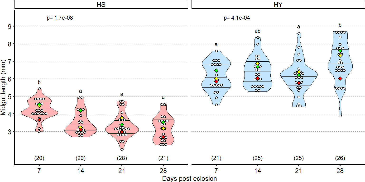
4.2.4 Figure 4S1D
Midgut size is a plastic, diet-dependent trait. Midguts of flies shifted between HS or HY can reversibly grow throughout 21 days. Statistical comparison is vs pre-shift measurement.
Length_shift_growth =
d[["4C, 4S1D"]]%>%
select(-Total.PH3)%>%
mutate(Total_Length_mm = Total.L/1000)%>%
mutate_if(is.character,as.factor)%>%
mutate_if(is.integer,as.factor)%>%
dplyr::rename(Day_of_treatment=Day)%>%
as.data.frame()%>%
mutate(Dday=fct_relevel(Dday,"Shift Day 7","Shift Day 14","Shift Day 21"))
Sample_size=
Length_shift_growth%>%
group_by(Dday,Diet)%>%
summarise(Sample_size=n())
###Stats
# Day 7
tmp= subset(Length_shift_growth,Dday=="Shift Day 7")
mod.gen = fitme(log(Total_Length_mm) ~ Diet + (1 | Repeat), data = tmp)
shapiro.test(residuals(mod.gen))
Shapiro-Wilk normality test
data: residuals(mod.gen)
W = 0.98038, p-value = 0.6352bptest(log(Total_Length_mm) ~ Diet + (1 / Repeat), data = tmp)
studentized Breusch-Pagan test
data: log(Total_Length_mm) ~ Diet + (1/Repeat)
BP = 0.59118, df = 1, p-value = 0.442mod.gen1 = fitme(log(Total_Length_mm) ~ 1 + (1 | Repeat), data = tmp)
test = anova(mod.gen, mod.gen1)
Chi2_LRT_growth = 2*(mod.gen$APHLs[["p_v"]]-mod.gen1$APHLs[["p_v"]])
tab_stat = data.frame(Comparison = as.character(paste(("HS Day 7 vs HS to HY Day 14"))),
Dday = as.character(paste("Shift Day 7")),
Rep = nlevels(tmp$Repeat),
chi2_LR = round(as.numeric(test$basicLRT$chi2_LR), digits = 2),
intercept = format(mod.gen$fixef[1],digits=3),
estimate = format(mod.gen$fixef[2],digits=3),
df = as.numeric(test$basicLRT$df),
Pvalue = as.numeric(format(pchisq(Chi2_LRT_growth,df=1,lower.tail = F),digits=2)))
tab_stat_7 = tab_stat
# Day 14
tmp= subset(Length_shift_growth,Dday=="Shift Day 14")
mod.gen = fitme(log(Total_Length_mm) ~ Diet + (1 | Repeat), data = tmp)
shapiro.test(residuals(mod.gen))
Shapiro-Wilk normality test
data: residuals(mod.gen)
W = 0.95853, p-value = 0.1396bptest(log(Total_Length_mm) ~ Diet + (1 / Repeat), data = tmp)
studentized Breusch-Pagan test
data: log(Total_Length_mm) ~ Diet + (1/Repeat)
BP = 5.1346, df = 1, p-value = 0.02345mod.gen1 = fitme(log(Total_Length_mm) ~ 1 + (1 | Repeat), data = tmp)
test = anova(mod.gen, mod.gen1)
Chi2_LRT_growth = 2*(mod.gen$APHLs[["p_v"]]-mod.gen1$APHLs[["p_v"]])
tab_stat = data.frame(Comparison = as.character(paste(("HS Day 14 vs HS to HY Day 21"))),
Dday = as.character(paste("Shift Day 14")),
Rep = nlevels(tmp$Repeat),
chi2_LR = round(as.numeric(test$basicLRT$chi2_LR), digits = 2),
intercept = format(mod.gen$fixef[1],digits=3),
estimate = format(mod.gen$fixef[2],digits=3),
df = as.numeric(test$basicLRT$df),
Pvalue = as.numeric(format(pchisq(Chi2_LRT_growth,df=1,lower.tail = F),digits=2)))
tab_stat_14 = tab_stat
# Day 21
tmp= subset(Length_shift_growth,Dday=="Shift Day 21")
mod.gen = fitme(log(Total_Length_mm) ~ Diet + (1 | Repeat), data = tmp)
shapiro.test(residuals(mod.gen))
Shapiro-Wilk normality test
data: residuals(mod.gen)
W = 0.97628, p-value = 0.346bptest(log(Total_Length_mm) ~ Diet + (1 / Repeat), data = tmp)
studentized Breusch-Pagan test
data: log(Total_Length_mm) ~ Diet + (1/Repeat)
BP = 0.19389, df = 1, p-value = 0.6597mod.gen1 = fitme(log(Total_Length_mm) ~ 1 + (1 | Repeat), data = tmp)
test = anova(mod.gen, mod.gen1)
Chi2_LRT_growth = 2*(mod.gen$APHLs[["p_v"]]-mod.gen1$APHLs[["p_v"]])
tab_stat = data.frame(Comparison = as.character(paste(("HS Day 21 vs HS to HY Day 28"))),
Dday = as.character(paste("Shift Day 21")),
Rep = nlevels(tmp$Repeat),
chi2_LR = round(as.numeric(test$basicLRT$chi2_LR), digits = 2),
intercept = format(mod.gen$fixef[1],digits=3),
estimate = format(mod.gen$fixef[2],digits=3),
df = as.numeric(test$basicLRT$df),
Pvalue = as.numeric(format(pchisq(Chi2_LRT_growth,df=1,lower.tail = F),digits=2)))
tab_stat_21 = tab_stat
tab_stat=rbind(tab_stat_7,tab_stat_14,tab_stat_21)
tab_stat$sig = ifelse(tab_stat$Pvalue < 0.05 & tab_stat$Pvalue > 0.01, "*",
ifelse(tab_stat$Pvalue < 0.01 & tab_stat$Pvalue > 0.001, "**",
ifelse(tab_stat$Pvalue < 0.001, "***", "")))
tab_stat%>%
kable(col.names = c("Comparison", "Shift day", "Replicates", "Chi2","Intercept","Estimate","df" ,"p-value","Signif."),row.names = FALSE) %>% add_header_above(c("log(Total_Length_mm) ~ Diet + (1 | Repeat)" = 9))%>%
kable_styling(bootstrap_options = c("striped", "hover", "condensed"), full_width = F)| Comparison | Shift day | Replicates | Chi2 | Intercept | Estimate | df | p-value | Signif. |
|---|---|---|---|---|---|---|---|---|
| HS Day 7 vs HS to HY Day 14 | Shift Day 7 | 3 | 47.53 | 1.43 | 0.284 | 1 | 0 | *** |
| HS Day 14 vs HS to HY Day 21 | Shift Day 14 | 3 | 51.25 | 1.24 | 0.412 | 1 | 0 | *** |
| HS Day 21 vs HS to HY Day 28 | Shift Day 21 | 3 | 54.31 | 1.19 | 0.497 | 1 | 0 | *** |
tab_stat=
tab_stat%>%
mutate_if(is.character,as.factor)%>%
as.data.frame()%>%
mutate(Dday=fct_relevel(Dday,"Shift Day 7","Shift Day 14","Shift Day 21"))
### Plot
Treatment.status = c("Shift\nDay 7","Shift\nDay 14","Shift\nDay 21")
names(Treatment.status) = c("Shift Day 7", "Shift Day 14","Shift Day 21")
z=max(Length_shift_growth$Total_Length_mm, na.rm = TRUE)
Plot_Fig4S1D=
ggplot(Length_shift_growth, aes(x = Diet, y = Total_Length_mm))+
geom_violin(aes(fill = Diet), draw_quantiles = c(0.25, 0.5, 0.75), colour = "black", size = 0.2,adjust = 0.8) +
geom_dotplot( colour = "black", fill = "white", binaxis = "y", stackdir = "center", binwidth = z/60) +
facet_grid(. ~ Dday,labeller=labeller(Dday=Treatment.status) )+
geom_text(data = Sample_size, mapping = aes(x = Diet, y = 1.6, label = paste("(",Sample_size,")",sep="")),size=3)+
geom_signif(data = tab_stat, aes(xmin = 1, xmax = 2, annotations = formatC(paste("p=",Pvalue), digits = 2), y_position = 9), textsize = 2.5, vjust = -0.2, manual = TRUE)+
scale_fill_manual(limits=c("HS","HStoHY"),
values=cbbHS_HStoHY)+
scale_x_discrete("",
limits=c("HS","HStoHY"),
labels=c("HS","HS to HY"))+
scale_y_continuous("Midgut length (mm)",
limits=c(1.5,9.5),
breaks=seq(2,8,by=1))+
stat_summary(fun = mean, geom = "point", size = 2.5, shape = 18,aes(group=Repeat, colour = Repeat)) +
stat_summary(fun = mean, geom = "point", size = 3, shape = 18, colour = "black", aes(group = Repeat)) +
stat_summary(fun = mean, geom = "point", size = 2, shape = 18, aes(group = Repeat, colour = Repeat)) +
scale_color_manual(values = palette_mean) +
theme(panel.grid.major.y = element_line(colour = grey(0.45), linetype = "dashed", size = 0.2),
panel.background = element_blank(),
axis.title.x = element_text(size=Smallfont,colour="black"),
axis.title.y = element_text(size=Smallfont,colour="black"),
axis.line.x = element_line(colour="black",size=0.75),
axis.line.y = element_line(colour="black",size=0.75),
axis.ticks.x = element_line(size = 0.75),
axis.ticks.y = element_line(size = 0.75),
axis.text.x = element_text(size=Smallfont,colour="black",angle=30,hjust=1),
axis.text.y = element_text(size=Smallfont,colour="black"),
plot.margin = unit(Margin, "cm"),
legend.direction = "vertical",
legend.box = "horizontal",
legend.position = "none",
legend.key.height = unit(0.4, "cm"),
legend.key.width= unit(0.6, "cm"),
legend.title = element_text(face="italic",size=Smallfont),
legend.key = element_rect(colour = 'white', fill = "white", linetype='dashed'),
legend.text = element_text(size=SuperSmallfont),
legend.background = element_rect(fill=NA),
strip.text.x = element_text(size = Smallfont, colour = "black", margin = margin(t = 2, r = 0, b = 2, l = 0)),
strip.text.y = element_text(size = Smallfont, colour = "black", margin = margin(t = 2, r = 0, b = 2, l = 0)),
strip.background = element_rect(fill=NA, colour="black"),
strip.placement="outside")
Plot_Fig4S1D
4.2.5 Figure 4S1E
Midgut size is a plastic, diet-dependent trait. Midguts of flies shifted between HS or HY can reversibly shrink throughout 21 days. Statistical comparison is vs pre-shift measurement.
Length_shift_Shrink =
d[["4C', 4S1D'"]]%>%
select(-Total.PH3)%>%
mutate(Total_Length_mm = Total.L/1000)%>%
mutate_if(is.character,as.factor)%>%
mutate_if(is.integer,as.factor)%>%
dplyr::rename(Day_of_treatment=Day)%>%
as.data.frame()%>%
mutate(Dday=fct_relevel(Dday,"Shift Day 7","Shift Day 14","Shift Day 21"))
Sample_size=
Length_shift_Shrink%>%
group_by(Dday,Diet)%>%
summarise(Sample_size=n())
###Stats
# Day 7
tmp= subset(Length_shift_Shrink,Dday=="Shift Day 7")
mod.gen = fitme(log(Total_Length_mm) ~ Diet + (1 | Repeat), data = tmp)
shapiro.test(residuals(mod.gen))
Shapiro-Wilk normality test
data: residuals(mod.gen)
W = 0.96958, p-value = 0.2925bptest(log(Total_Length_mm) ~ Diet + (1 / Repeat), data = tmp)
studentized Breusch-Pagan test
data: log(Total_Length_mm) ~ Diet + (1/Repeat)
BP = 0.0069323, df = 1, p-value = 0.9336mod.gen1 = fitme(log(Total_Length_mm) ~ 1 + (1 | Repeat), data = tmp)
test = anova(mod.gen, mod.gen1)
Chi2_LRT_growth = 2*(mod.gen$APHLs[["p_v"]]-mod.gen1$APHLs[["p_v"]])
tab_stat = data.frame(Comparison = as.character(paste(("HS Day 7 vs HS to HY Day 14"))),
Dday = as.character(paste("Shift Day 7")),
Rep = nlevels(tmp$Repeat),
chi2_LR = round(as.numeric(test$basicLRT$chi2_LR), digits = 2),
intercept = format(mod.gen$fixef[1],digits=3),
estimate = format(mod.gen$fixef[2],digits=3),
df = as.numeric(test$basicLRT$df),
Pvalue = as.numeric(format(pchisq(Chi2_LRT_growth,df=1,lower.tail = F),digits=2)))
tab_stat_7 = tab_stat
# Day 14
tmp= subset(Length_shift_Shrink,Dday=="Shift Day 14")
mod.gen = fitme(log(Total_Length_mm) ~ Diet + (1 | Repeat), data = tmp)
shapiro.test(residuals(mod.gen))
Shapiro-Wilk normality test
data: residuals(mod.gen)
W = 0.9797, p-value = 0.6218bptest(log(Total_Length_mm) ~ Diet + (1 / Repeat), data = tmp)
studentized Breusch-Pagan test
data: log(Total_Length_mm) ~ Diet + (1/Repeat)
BP = 2.953, df = 1, p-value = 0.08572mod.gen1 = fitme(log(Total_Length_mm) ~ 1 + (1 | Repeat), data = tmp)
test = anova(mod.gen, mod.gen1)
Chi2_LRT_growth = 2*(mod.gen$APHLs[["p_v"]]-mod.gen1$APHLs[["p_v"]])
tab_stat = data.frame(Comparison = as.character(paste(("HS Day 14 vs HS to HY Day 21"))),
Dday = as.character(paste("Shift Day 14")),
Rep = nlevels(tmp$Repeat),
chi2_LR = round(as.numeric(test$basicLRT$chi2_LR), digits = 2),
intercept = format(mod.gen$fixef[1],digits=3),
estimate = format(mod.gen$fixef[2],digits=3),
df = as.numeric(test$basicLRT$df),
Pvalue = as.numeric(format(pchisq(Chi2_LRT_growth,df=1,lower.tail = F),digits=2)))
tab_stat_14 = tab_stat
# Day 21
tmp= subset(Length_shift_Shrink,Dday=="Shift Day 21")
mod.gen = fitme(log(Total_Length_mm) ~ Diet + (1 | Repeat), data = tmp)
shapiro.test(residuals(mod.gen))
Shapiro-Wilk normality test
data: residuals(mod.gen)
W = 0.9841, p-value = 0.7537bptest(log(Total_Length_mm) ~ Diet + (1 / Repeat), data = tmp)
studentized Breusch-Pagan test
data: log(Total_Length_mm) ~ Diet + (1/Repeat)
BP = 0.11454, df = 1, p-value = 0.735mod.gen1 = fitme(log(Total_Length_mm) ~ 1 + (1 | Repeat), data = tmp)
test = anova(mod.gen, mod.gen1)
Chi2_LRT_growth = 2*(mod.gen$APHLs[["p_v"]]-mod.gen1$APHLs[["p_v"]])
tab_stat = data.frame(Comparison = as.character(paste(("HS Day 21 vs HS to HY Day 28"))),
Dday = as.character(paste("Shift Day 21")),
Rep = nlevels(tmp$Repeat),
chi2_LR = round(as.numeric(test$basicLRT$chi2_LR), digits = 2),
intercept = format(mod.gen$fixef[1],digits=3),
estimate = format(mod.gen$fixef[2],digits=3),
df = as.numeric(test$basicLRT$df),
Pvalue = as.numeric(format(pchisq(Chi2_LRT_growth,df=1,lower.tail = F),digits=2)))
tab_stat_21 = tab_stat
tab_stat=rbind(tab_stat_7,tab_stat_14,tab_stat_21)
tab_stat$sig = ifelse(tab_stat$Pvalue < 0.05 & tab_stat$Pvalue > 0.01, "*",
ifelse(tab_stat$Pvalue < 0.01 & tab_stat$Pvalue > 0.001, "**",
ifelse(tab_stat$Pvalue < 0.001, "***", "")))
tab_stat%>%
kable(col.names = c("Comparison","Shift day", "Replicates", "Chi2","Intercept","Estimate","df" ,"p-value","Signif."),row.names = FALSE) %>% add_header_above(c("log(Total length) ~ Day + Diet + (1 | Repeat)" = 9))%>%
kable_styling(bootstrap_options = c("striped", "hover", "condensed"), full_width = F)| Comparison | Shift day | Replicates | Chi2 | Intercept | Estimate | df | p-value | Signif. |
|---|---|---|---|---|---|---|---|---|
| HS Day 7 vs HS to HY Day 14 | Shift Day 7 | 3 | 43.00 | 1.8 | -0.349 | 1 | 0.0e+00 | *** |
| HS Day 14 vs HS to HY Day 21 | Shift Day 14 | 3 | 38.48 | 1.86 | -0.366 | 1 | 0.0e+00 | *** |
| HS Day 21 vs HS to HY Day 28 | Shift Day 21 | 3 | 21.89 | 1.8 | -0.251 | 1 | 2.9e-06 | *** |
tab_stat=
tab_stat%>%
mutate_if(is.character,as.factor)%>%
as.data.frame()%>%
mutate(Dday=fct_relevel(Dday,"Shift Day 7","Shift Day 14","Shift Day 21"))
### Plot
Treatment.status = c("Shift\nDay 7","Shift\nDay 14","Shift\nDay 21")
names(Treatment.status) = c("Shift Day 7", "Shift Day 14","Shift Day 21")
z=max(Length_shift_Shrink$Total_Length_mm, na.rm = TRUE)
Plot_Fig4S1E=
ggplot(Length_shift_Shrink, aes(x = Diet, y = Total_Length_mm))+
geom_violin(aes(fill = Diet), draw_quantiles = c(0.25, 0.5, 0.75), colour = "black", size = 0.2,adjust = 0.8) +
geom_dotplot( colour = "black", fill = "white", binaxis = "y", stackdir = "center", binwidth = 0.15) +
facet_grid(. ~ Dday,labeller=labeller(Dday=Treatment.status) )+
geom_text(data = Sample_size, mapping = aes(x = Diet, y = 1.6, label = paste("(",Sample_size,")",sep="")),size=3)+
geom_signif(data = tab_stat, aes(xmin = 1, xmax = 2, annotations = formatC(paste("p=",Pvalue), digits = 2), y_position = 9), textsize = 2.5, vjust = -0.2, manual = TRUE)+
scale_fill_manual(limits=c("HY","HYtoHS"),
values=cbbHY_HYtoHS)+
scale_x_discrete("",
limits=c("HY","HYtoHS"),
labels=c("HY","HY to HS"))+
scale_y_continuous("Midgut length (mm)",
limits=c(1.5,9.5),
breaks=seq(2,8,by=1))+
stat_summary(fun = mean, geom = "point", size = 2.5, shape = 18,aes(group=Repeat, colour = Repeat)) +
stat_summary(fun = mean, geom = "point", size = 3, shape = 18, colour = "black", aes(group = Repeat)) +
stat_summary(fun = mean, geom = "point", size = 2, shape = 18, aes(group = Repeat, colour = Repeat)) +
scale_color_manual(values = palette_mean) +
theme(panel.grid.major.y = element_line(colour = grey(0.45), linetype = "dashed", size = 0.2),
panel.background = element_blank(),
axis.title.x = element_text(size=Smallfont,colour="black"),
axis.title.y = element_text(size=Smallfont,colour="black"),
axis.line.x = element_line(colour="black",size=0.75),
axis.line.y = element_line(colour="black",size=0.75),
axis.ticks.x = element_line(size = 0.75),
axis.ticks.y = element_line(size = 0.75),
axis.text.x = element_text(size=Smallfont,colour="black",angle=30,hjust=1),
axis.text.y = element_text(size=Smallfont,colour="black"),
plot.margin = unit(Margin, "cm"),
legend.direction = "vertical",
legend.box = "horizontal",
legend.position = "none",
legend.key.height = unit(0.4, "cm"),
legend.key.width= unit(0.6, "cm"),
legend.title = element_text(face="italic",size=Smallfont),
legend.key = element_rect(colour = 'white', fill = "white", linetype='dashed'),
legend.text = element_text(size=SuperSmallfont),
legend.background = element_rect(fill=NA),
strip.text.x = element_text(size = Smallfont, colour = "black", margin = margin(t = 2, r = 0, b = 2, l = 0)),
strip.text.y = element_text(size = Smallfont, colour = "black", margin = margin(t = 2, r = 0, b = 2, l = 0)),
strip.background = element_rect(fill=NA, colour="black"),
strip.placement="outside")
Plot_Fig4S1E
4.2.6 Figure 4S1F
ISC proliferation is promoted by yeast and antagonized by sugar. Cell proliferation (pH3 stain) is impeded by dietary sucrose, and increased by yeast, similar to total midgut length (Figure 2A). Plots showing counts of pH3+ cells as a function of ingested yeast and sucrose.
tab_nutri_geo_PH3 =
d[["4 - S1F"]]
jpeg(filename = "Plot_Fig4-S1F.jpeg",
res = 600,
width = 5, height = 4, units = 'in' )
par(cex=1, mar = c(4.5, 4.5, 1, 3))
with(tab_nutri_geo_PH3, geomPlotta(x = Sucrose.in.Diet, y = Yeast.in.Diet, z = Ph3.Total, alf = 1, xlim = c(-10, 300), ylim = c(-10, 300), xlab = "Sucrose in diet (g/L)", ylab = "Yeast in diet (g/L)", frame.plot= FALSE, cex.lab=1.2, cex.axis =1, las=1, labcex=1, asp=1))img4S1F = readImage("F:/Dropbox/Github/Bonfini_eLife_2021/data/Plot_Fig4-S1F.jpeg")
gob_imageFig4S1F = rasterGrob(img4S1F)
grid.draw(gob_imageFig4S1F)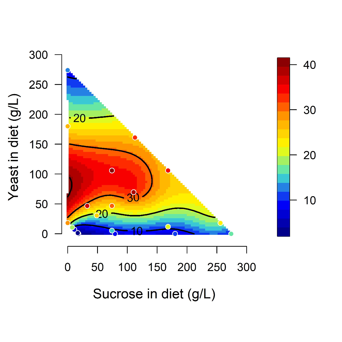
4.2.7 Figure 4S1G
Plots showing pH3+ cell counts increase with dietary yeast, with an optimum around HY diet. Increasing sucrose reduces counts of pH3+ cells.
tab_nutri_geo_PH3 =
d[["4 - S1F"]]
tab_nutri_geo_PH32 <- tab_nutri_geo_PH3 %>%
group_by(concatenate) %>%
summarize(Calories.ingested = mean(Calories.ingested),
Ph3.Total = mean(Ph3.Total),
Yeast.ingested = mean(Yeast.ingested),
Sucrose.ingested = mean(Sucrose.ingested))
graph <- ggplot(tab_nutri_geo_PH32, aes(x=Sucrose.ingested, y=Yeast.ingested))
Plot_Fig4S1G=
graph + geom_point(aes(size=Calories.ingested, fill=Ph3.Total), stroke=1, shape=21, color="black") +
scale_size(range = c(1,5)) +
scale_fill_viridis_c() +
theme(plot.title= element_text(hjust = 0.5))+
scale_x_continuous("Sucrose ingested (g/L x Absorbance)",
limits=c(-5,160),
breaks=seq(0,160,by=25))+
scale_y_continuous("Yeast ingested (g/L x Absorbance)",
limits=c(-5,50),
breaks=seq(0,50,by=10))+
scale_size_continuous(range = c(1,5)) +
theme(panel.background = element_blank(),
panel.grid.major = element_line(colour = "black",linetype=3),
axis.title.x = element_text(size=Smallfont,colour="black"),
axis.title.y = element_text(size=Smallfont,colour="black"),
axis.line.x = element_line(colour="black",size=0.75),
axis.line.y = element_line(colour="black",size=0.75),
axis.ticks.x = element_line(size = 0.75),
axis.ticks.y = element_line(size = 0.75),
axis.text.x = element_text(size=Smallfont,colour="black"),
axis.text.y = element_text(size=Smallfont,colour="black"),
plot.margin = unit(c(0,0,0,0.5), "cm"),
legend.direction = "horizontal",
legend.box = "vertical",
legend.position = c(0.75,0.79),
legend.key.height = unit(0.3, "cm"),
legend.key.width= unit(0.3, "cm"),
legend.title = element_text(face="italic",size=Smallfont),
legend.key = element_rect(colour = 'white', fill = "white", linetype='dashed'),
legend.text = element_text(size=SuperSmallfont),
legend.box.background = element_rect(fill="white", colour ="black"),
legend.spacing.y = unit(0, "cm"))+
labs(fill = expression(paste("pH3" ^ "+", " cells")), size = "Calories
ingested", vjust="center" )
Plot_Fig4S1G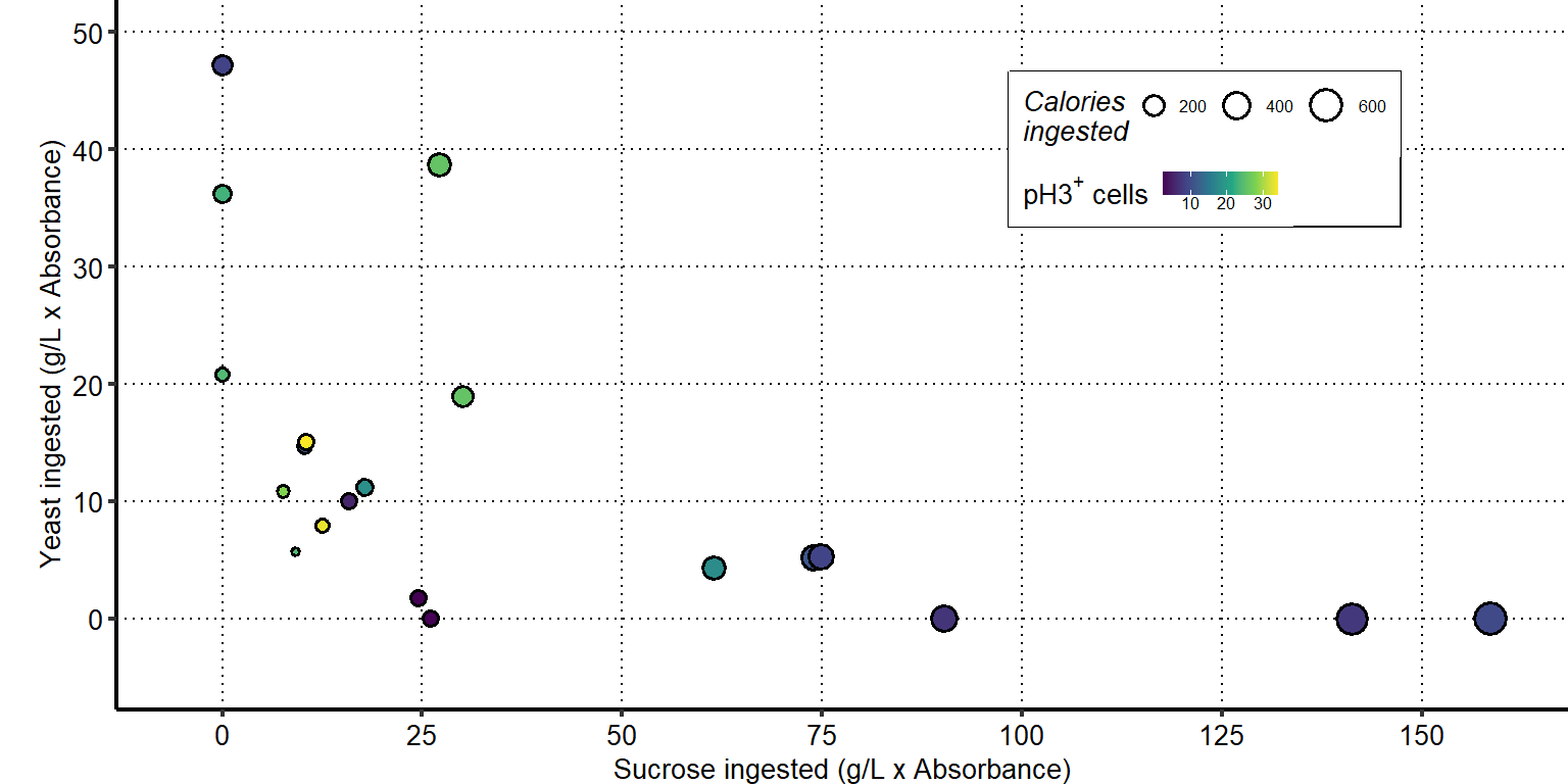
##Export Figure 4S1
4.3 Figure 4 - supplementary 2
4.3.1 Figure 4S2A
Illustration of the cell loss assay (Figure 4G - L). A pulse of RU486 for 3 days marks all ECs and EBs through 5966GS>His-2BRFP. Flies were dissected at 2 and 16-days after cessation of hormone pulse.
img4S2A = readImage("F:/Dropbox/Github/Bonfini_eLife_2021/data/4 - S2A.jpg")
gob_imageFig4S2A = rasterGrob(img4S2A)
grid.draw(gob_imageFig4S2A)
4.3.2 Figure 4S2B
His2B-RFP is highly stable on both HS and HY diets on tissues not undergoing turnover in a manner similar to the midgut. We assayed the stability of the His2B-RFP by driving it through an ActGS driver, in the crop and hindgut in the same timeline as the experiment presented in Figure 4K. In both organs, we found a high degree of cells marked by His2B-RFP, and on both diets, at both the initial timepoint and after 14 days from the start of the chase. Day of dissection at the bottom of the chart are relative to start of pulse chase.
tab_Hisstab_rev =
d[["4S2B"]]%>%
mutate_at(vars(!starts_with("RFP")),as.factor)
###Stats
#Crop
tmp = subset(tab_Hisstab_rev , Tissue%in%c("Crop"))
mod.gen = fitme((RFP.Dapi) ~ Day * Diet + (1 | Repeat),data = tmp)
shapiro.test(residuals(mod.gen))
Shapiro-Wilk normality test
data: residuals(mod.gen)
W = 0.97787, p-value = 0.3043bptest((RFP.Dapi) ~ Day * Diet + (1 / Repeat),data = tmp)
studentized Breusch-Pagan test
data: (RFP.Dapi) ~ Day * Diet + (1/Repeat)
BP = 11.797, df = 3, p-value = 0.008111mod.gen1 = fitme((RFP.Dapi) ~ Day + Diet + (1 | Repeat),data = tmp)
test = anova(mod.gen, mod.gen1)
test chi2_LR df p_value
p_v 0.3811947 1 0.5369646Chi2_LRT_growth = 2*(mod.gen$APHLs[["p_v"]]-mod.gen1$APHLs[["p_v"]])
tab_stat = data.frame(Tissue = as.character(paste("Crop")),
Rep = nlevels(tmp$Repeat),
chi2_LR = round(as.numeric(test$basicLRT$chi2_LR), digits = 2),
intercept = format(mod.gen$fixef[1],digits=3),
estimate = format(mod.gen$fixef[2],digits=3),
df = as.numeric(test$basicLRT$df),
Pvalue = as.numeric(format(pchisq(Chi2_LRT_growth,df=1,lower.tail = F),digits=1,scientific=F)))
tab_stat_Crop=tab_stat
#Hindgut
tmp = subset(tab_Hisstab_rev , Tissue%in%c("Hindgut"))
mod.gen = fitme((RFP.Dapi) ~ Day * Diet + (1 | Repeat),data = tmp)
shapiro.test(residuals(mod.gen))
Shapiro-Wilk normality test
data: residuals(mod.gen)
W = 0.63759, p-value = 2.106e-12bptest((RFP.Dapi) ~ Day * Diet + (1 / Repeat),data = tmp)
studentized Breusch-Pagan test
data: (RFP.Dapi) ~ Day * Diet + (1/Repeat)
BP = 1.526, df = 3, p-value = 0.6763mod.gen1 = fitme((RFP.Dapi) ~ Day + Diet + (1 | Repeat),data = tmp)
test = anova(mod.gen, mod.gen1)
test chi2_LR df p_value
p_v 0.008096241 1 0.9283038Chi2_LRT_growth = 2*(mod.gen$APHLs[["p_v"]]-mod.gen1$APHLs[["p_v"]])
tab_stat = data.frame(Tissue = as.character(paste("Hindgut")),
Rep = nlevels(tmp$Repeat),
chi2_LR = round(as.numeric(test$basicLRT$chi2_LR), digits = 2),
intercept = format(mod.gen$fixef[1],digits=3),
estimate = format(mod.gen$fixef[2],digits=3),
df = as.numeric(test$basicLRT$df),
Pvalue = as.numeric(format(pchisq(Chi2_LRT_growth,df=1,lower.tail = F),digits=1,scientific=F)))
tab_stat_Hindgut=tab_stat
#Table
tab_stat=rbind(tab_stat_Crop,tab_stat_Hindgut)
tab_stat$padj = as.numeric(format(p.adjust(tab_stat$Pvalue, method = "BH"),digits=2,scientific =F))
tab_stat$sig = ifelse(tab_stat$padj < 0.05 & tab_stat$padj > 0.01, "*",
ifelse(tab_stat$padj < 0.01 & tab_stat$padj > 0.001, "**",
ifelse(tab_stat$padj < 0.001, "***", "")))
tab_stat%>%
kable(col.names = c("Variable", "Replicates", "Chi2","Intercept","Estimate","df" ,"p-value","p-value adjusted","Signif."),row.names = FALSE) %>%
add_header_above(c("(RFP/Dapi) ~ Diet + Genotype + Diet : Genotype + (1 | Repeat)" = 9))%>%
kable_styling(bootstrap_options = c("striped", "hover", "condensed"), full_width = F)| Variable | Replicates | Chi2 | Intercept | Estimate | df | p-value | p-value adjusted | Signif. |
|---|---|---|---|---|---|---|---|---|
| Crop | 3 | 0.38 | 84.4 | 4.21 | 1 | 0.5 | 0.9 | |
| Hindgut | 3 | 0.01 | 99.1 | -0.00928 | 1 | 0.9 | 0.9 |
tab_stat_rev_Hisstab=tab_stat
tab_stat_rev_Hisstab$Diet = "HY"
Sample_size=
tab_Hisstab_rev%>%
group_by(Diet, Day, Tissue)%>%
summarise(Sample_size=n())
### Plot
Limits = c("0","14")
Plot_Fig4S2B=
ggplot(tab_Hisstab_rev, aes(x = Day, y = RFP.Dapi))+
geom_violin(aes(fill = Diet), draw_quantiles = c(0.25, 0.5, 0.75), colour = "black", size = 0.2,adjust = 0.8) +
geom_dotplot( colour = "black", fill = "white", binaxis = "y", stackdir = "center", binwidth = 4) +
facet_grid(Tissue ~ Diet,labeller=label_parsed)+
geom_text(data = Sample_size, mapping = aes(x = Day, y = 10, label = paste("(",Sample_size,")",sep="")),size=3)+
scale_fill_manual(limits=c("HS","HY"),
values=c("#FFB4B4","#C3E6FC"))+
scale_x_discrete("Day of dissection post RU486 pulse",
limits=Limits,
labels=c("0","14"))+
scale_y_continuous(expression(paste("RFP pos. cells / Total cells %")),
limits=c(0,110),
breaks=seq(0,100,by=20))+
stat_summary(fun = mean, geom = "point", size = 3, shape = 18, colour = "black", aes(group = Repeat)) +
stat_summary(fun = mean, geom = "point", size = 2, shape = 18, aes(group = Repeat, colour = Repeat)) +
stat_summary(fun = mean, colour = "black", geom = "line", aes(group = Repeat)) +
scale_color_manual(values = palette_mean) +
theme(panel.grid.major.y = element_line(colour = grey(0.45), linetype = "dashed", size = 0.2),
panel.background = element_blank(),
axis.title.x = element_text(size=Smallfont,colour="black"),
axis.title.y = element_text(size=Smallfont,colour="black", margin = margin(t = 0, r = 0, b = 0, l = 0) ),
axis.line.x = element_line(colour="black",size=0.75),
axis.line.y = element_line(colour="black",size=0.75),
axis.ticks.x = element_line(size = 0.75),
axis.ticks.y = element_line(size = 0.75),
axis.text.x = element_text(size=Smallfont,colour="black"),
axis.text.y = element_text(size=Smallfont,colour="black"),
plot.margin = unit(Margin, "cm"),
legend.direction = "vertical",
legend.box = "horizontal",
legend.position = "none",
legend.key.height = unit(0.4, "cm"),
legend.key.width= unit(0.6, "cm"),
legend.title = element_text(face="italic",size=Smallfont),
legend.key = element_rect(colour = 'white', fill = "white", linetype='dashed'),
legend.text = element_text(size=SuperSmallfont),
legend.background = element_rect(fill=NA),
strip.text = element_text(size =Smallfont-2, colour = "black",face="italic", margin = margin(t = 2, r = 1, b = 2, l = 1)),
strip.background = element_rect(fill=NA, colour="black"),
strip.placement="outside")
Plot_Fig4S2B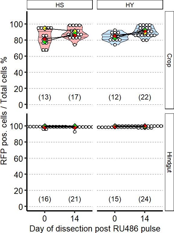
4.3.3 Figure 4S2C
Cell loss assay performed at 5 days post start of chase shows limited cell loss in HY to HY condition. Number of ECs in the posterior midgut, both marked (Red, old ECs) and unmarked (Blue, new ECs) by RFP, error bars are SE from 3 repeats.
tab_prop_cell_RFP_kin =
d[["4S2C"]]%>%
mutate_if(is.character,as.factor)%>%
mutate_if(is.integer,as.factor)%>%
mutate(Post.Dapi.Number = (Post.Dapi.Number)*2)%>%
mutate(Post.RFP.Number = (Post.RFP.Number)*2)%>%
mutate(Post.NonRFP.Number = (Post.Dapi.Number - Post.RFP.Number))%>%
group_by(Day, Diet, CG, Experiment)%>%
summarise(mean_RFP_positive=mean(Post.RFP.Number,na.rm=T),
se_RFP_positive=se(Post.RFP.Number),
mean_RFP_negative=mean(Post.NonRFP.Number,na.rm=T),
se_RFP_negative=se(Post.NonRFP.Number))%>%
mutate(group=paste(Diet,Experiment,sep="_"))%>%
as.data.frame()
attach(tab_prop_cell_RFP_kin)
for (i in 1:length(Experiment)){
tab_prop_cell_RFP_kin$se_proportionGraphPlus_pos[i] = mean_RFP_positive[i]+se_RFP_positive[i]
tab_prop_cell_RFP_kin$se_proportionGraphMinus_pos[i] = mean_RFP_positive[i]-se_RFP_positive[i]
tab_prop_cell_RFP_kin$se_proportionGraphPlus_neg[i] = mean_RFP_positive[i]+mean_RFP_negative[i]+se_RFP_negative[i]
tab_prop_cell_RFP_kin$se_proportionGraphMinus_neg[i] = mean_RFP_positive[i]+mean_RFP_negative[i]-se_RFP_negative[i]
}
tmp1 = tab_prop_cell_RFP_kin[,c("Day", "Diet", "CG", "Experiment","mean_RFP_positive", "se_RFP_positive","se_proportionGraphPlus_pos", "se_proportionGraphMinus_pos")]
tmp1$RFP="Positive"
tmp1=dplyr::rename(tmp1,mean_RFP = mean_RFP_positive,
se_RFP = se_RFP_positive,
se_proportionGraphPlus =se_proportionGraphPlus_pos,
se_proportionGraphMinus= se_proportionGraphMinus_pos)
tmp2 = tab_prop_cell_RFP_kin[,c("Day", "Diet", "CG", "Experiment","mean_RFP_negative", "se_RFP_negative", "se_proportionGraphMinus_neg" ,"se_proportionGraphPlus_neg")]
tmp2$RFP="Negative"
tmp2=dplyr::rename(tmp2,mean_RFP = mean_RFP_negative,
se_RFP = se_RFP_negative,
se_proportionGraphPlus =se_proportionGraphPlus_neg,
se_proportionGraphMinus= se_proportionGraphMinus_neg)
tab_prop_cell_RFP_kin = rbind(tmp1,tmp2)
tab_prop_cell_RFP_kin =
tab_prop_cell_RFP_kin%>%
mutate_if(is.numeric,round,0)%>%
mutate_if(is.character,as.factor)
levels(tab_prop_cell_RFP_kin$Diet) <- c("HS", "HS to HS" , "HS to HY", "HY", "HY to HS", "HY to HY")
Sample_size=
d[["4S2C"]]%>%
mutate_if(is.character,as.factor)%>%
mutate_if(is.integer,as.factor)%>%
group_by(Diet)%>%
summarise(Sample_size=n())
Sample_size$Experiment = c("G", "G", "G", "S", "S", "S")
levels(Sample_size$Diet) <- c("HS", "HS to HS" , "HS to HY", "HY", "HY to HS", "HY to HY")
Plot_Fig4S2C =
ggplot(tab_prop_cell_RFP_kin, aes(x=Diet, y=mean_RFP))+
geom_bar(stat="identity",aes(fill=RFP),color="black",width=.90)+
geom_errorbar(aes(ymin= se_proportionGraphMinus, ymax= se_proportionGraphPlus),width=0.25)+
geom_text(data = Sample_size, mapping = aes(x = Diet, y = 200, label = paste("(",Sample_size,")",sep="")),size=3)+
#facet_wrap(.~Experiment,scales="free_x")+
scale_fill_manual(name = "RFP labelling",
values=c("#3a5ecc","#cc0000"),
labels = c("Negative", "Positive"))+
scale_y_continuous("Number of cells (mean \u00B1se)",
limits=c(0,5800),
breaks=seq(0,5000,by=500))+
theme(
panel.grid.major.y = element_line(colour = grey(0.45), linetype = "dashed", size = 0.2),
panel.background = element_blank(),
axis.title.x = element_blank(),
axis.title.y = element_text(size=Smallfont,colour="black"),
axis.line.x = element_line(colour="black",size=0.75),
axis.line.y = element_line(colour="black",size=0.75),
axis.ticks.x = element_line(size = 0.75),
axis.ticks.y = element_line(size = 0.75),
axis.text.x = element_text(size=Smallfont,colour="black",angle=30,hjust=1),
axis.text.y = element_text(size=Smallfont,colour="black"),
plot.margin = unit(Margin, "cm"),
legend.direction = "vertical",
legend.box = "horizontal",
legend.position = c(0.2,0.87),
legend.key.height = unit(0.4, "cm"),
legend.key.width= unit(0.6, "cm"),
legend.title = element_text(face="italic",size=Smallfont),
legend.key = element_rect(colour = 'white', fill = "white", linetype='dashed'),
legend.text = element_text(size=Smallfont),
legend.background = element_rect(fill=NA),
strip.text = element_blank())
#strip.background = element_rect(fill=NA, colour="black"),
#strip.placement="outside")
Plot_Fig4S2C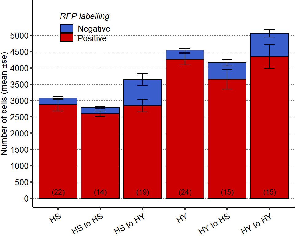
4.3.4 Figure 4S2D
Diet composition modulates cell replacement rate (cell/day). Bar chart was made using the same data as in Figure 4 K, L.
tab_relative_cell_rate_supp =
d[["4L, 4S2D"]]%>%
select(-starts_with("X"))%>%
drop_na()%>%
mutate_if(is.character,as.factor)%>%
group_by(Diet1, Experiment, Experiment2, GL)%>%
summarise(mean_Daily=mean(Daily,na.rm=T))%>%
mutate(group=paste(Diet1,Experiment,sep="_"))%>%
as.data.frame()
tab_relative_cell_rate_ratio =
tab_relative_cell_rate_supp%>%
group_by(Diet1,Experiment2)%>%
summarize(Ratio = round(mean_Daily[GL == "Gain"] / (-mean_Daily[GL == "Loss"]),2))%>%
mutate(GL="Loss")
levels(tab_relative_cell_rate_supp$Diet1) <- c("HS to HS" , "HS to HY", "HY to HS", "HY to HY")
levels(tab_relative_cell_rate_ratio$Diet1) <- c("HS to HS" , "HS to HY", "HY to HS", "HY to HY")
Plot_Fig4S2D =
ggplot(tab_relative_cell_rate_supp, aes(x = Diet1, y = mean_Daily, fill = GL))+
geom_bar(stat="identity",aes(fill=GL),color="black",width=.90)+
geom_hline(yintercept = 0)+
geom_text(data=tab_relative_cell_rate_ratio,mapping=aes(x=Diet1,y=-20,label=Ratio), color = "red")+
facet_grid(.~Experiment2,scales="free_x")+
scale_fill_manual(name = "Enterocyte",
values=c("palegreen", "moccasin"),
labels = c("Gain", "Loss"))+
scale_y_continuous("Cell rate (cell/ day)",
limits=c(-220,220),
breaks=seq(-200,200,by=50))+
theme(
panel.grid.major.y = element_line(colour = grey(0.45), linetype = "dashed", size = 0.2),
panel.background = element_blank(),
axis.title.x = element_blank(),
axis.title.y = element_text(size=Smallfont,colour="black"),
axis.line.x = element_line(colour="black",size=0.75),
axis.line.y = element_line(colour="black",size=0.75),
axis.ticks.x = element_line(size = 0.75),
axis.ticks.y = element_line(size = 0.75),
axis.text.x = element_text(size=Smallfont,colour="black",angle=30,hjust=1),
axis.text.y = element_text(size=Smallfont,colour="black"),
plot.margin = unit(Margin, "cm"),
legend.direction = "vertical",
legend.box = "horizontal",
legend.position = c(0.18,0.88),
legend.key.height = unit(0.4, "cm"),
legend.key.width= unit(0.6, "cm"),
legend.title = element_text(face="italic",size=Smallfont),
legend.key = element_rect(colour = 'white', fill = "white", linetype='dashed'),
legend.text = element_text(size=Smallfont),
legend.background = element_rect(fill=NA),
strip.text.x = element_text(size = Smallfont, colour = "black", margin = margin(t = 2, r = 0, b = 2, l = 0)),
strip.text.y = element_text(size = Smallfont, colour = "black", margin = margin(t = 2, r = 0, b = 2, l = 0)),
strip.background = element_rect(fill=NA, colour="black"),
strip.placement="outside")
Plot_Fig4S2D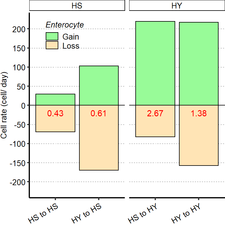
##Export Figure 4S2
5 Figure 5. Sugar uncouples ISC proliferation from niche signal expression by inducing translational stress
5.1 Figure 5 - main
5.1.1 Figure 5A
Diet influences midgut transcriptomes after an initial programmed developmental transition. The plot shows a PCA of the whole transcriptome, with means per diet per day ± standard error (3 repeats). Numbers on the plot represent the day of dissection from eclosion. Lines connect the datapoints sequentially (Day 0 to day 1, day 1 to day 2, and so on), and show the divergent transcriptomic trajectory followed by midguts on the two different diets from eclosion.
dataInd =
d[["gutGrowthDataIndex"]]%>%
mutate_if(is.character,as.factor)%>%
mutate_if(is.integer,as.factor)
#add string to direct to enumerated reads
dataInd$countFile = gsub(".fastq", "_sn.sam.count", dataInd$library)
dataInd$samp = paste("day",dataInd$day,"_diet",dataInd$diet,"_rep",dataInd$rep,sep="")
dataInd$expCond = factor(paste(dataInd$day, dataInd$diet, sep=""))
dataInd$dietCol = with( dataInd, ifelse(diet=="x", "#ff9595", ifelse(diet=="y", "#abefff", "#67ff67")) )
tab_read_RNAseq = d[["readTable"]]
geneID = rownames(tab_read_RNAseq) = tab_read_RNAseq$FBid
tab_read_RNAseq = tab_read_RNAseq[,2:ncol(tab_read_RNAseq)]
normCounts = d[["normCounts"]]
rownames(normCounts) = geneID
normCounts = normCounts[,2:ncol(normCounts)]
#pca without day 4
dataInd2 = droplevels(subset(dataInd, day!=4))
normCounts2 = normCounts[,dataInd$day!=4]
pca2 = prcomp(t(normCounts2))
summary(pca2)Importance of components:
PC1 PC2 PC3 PC4 PC5 PC6
Standard deviation 27.1902 19.9723 14.67551 13.46729 10.71975 9.34310
Proportion of Variance 0.2674 0.1443 0.07789 0.06559 0.04156 0.03157
Cumulative Proportion 0.2674 0.4116 0.48951 0.55510 0.59666 0.62823
PC7 PC8 PC9 PC10 PC11 PC12 PC13
Standard deviation 8.98836 8.74368 8.35311 8.18187 8.02046 7.7286 7.69699
Proportion of Variance 0.02922 0.02765 0.02523 0.02421 0.02326 0.0216 0.02143
Cumulative Proportion 0.65745 0.68510 0.71033 0.73454 0.75780 0.7794 0.80083
PC14 PC15 PC16 PC17 PC18 PC19 PC20
Standard deviation 7.55465 7.32756 7.21305 6.84985 6.72589 6.651 6.33040
Proportion of Variance 0.02064 0.01942 0.01882 0.01697 0.01636 0.016 0.01449
Cumulative Proportion 0.82147 0.84089 0.85970 0.87667 0.89303 0.909 0.92352
PC21 PC22 PC23 PC24 PC25 PC26 PC27
Standard deviation 6.22794 6.14888 6.0655 5.9721 5.81879 5.34384 6.139e-14
Proportion of Variance 0.01403 0.01367 0.0133 0.0129 0.01224 0.01033 0.000e+00
Cumulative Proportion 0.93755 0.95122 0.9645 0.9774 0.98967 1.00000 1.000e+00 #calculate means and SEs of the PCs
#without day 4
pcMns = aggregate(pca2$x ~ day * diet + dietCol, data=dataInd2, mean)
pcSEs = aggregate(pca2$x ~ day * diet + dietCol, data=dataInd2, function(x){sd(x)/sqrt(length(x))})
pcMns = droplevels(subset(pcMns, day!=4))
pcSEs = droplevels(subset(pcSEs, day!=4))
pcMns = pcMns[order(pcMns$day),]
pcSEs = pcSEs[order(pcSEs$day),]
pcMns = pcMns%>%
mutate_if(is.character,as.factor)%>%
select(day,diet,dietCol,PC1,PC2)%>%
as.data.frame()%>%
dplyr::rename(PC1_mean=PC1,
PC2_mean=PC2)
pcSEs = pcSEs%>%
mutate_if(is.character,as.factor)%>%
select(day,diet,dietCol,PC1,PC2)%>%
dplyr::rename(PC1_se=PC1,
PC2_se=PC2)
tab_PCA = left_join(pcMns,pcSEs)
tab_PCA$diet1 =ifelse(tab_PCA$diet=="x","#ff9595","#abefff")
tab_PCA$diet1[1]="#ff9595"
tab_PCA$diet2=ifelse(tab_PCA$diet=="y","#abefff","#ff9595")
tab_PCA$diet2[1]="#abefff"
tab_PCA=mutate_if(tab_PCA,is.character,as.factor)
tab_PCA$diet1= factor(tab_PCA$diet1,levels=c("#67ff67","#abefff","#ff9595"))
tab_PCA$diet2= factor(tab_PCA$diet2,levels=c("#67ff67","#abefff","#ff9595"))
Plot_Fig5A=
ggplot(tab_PCA,aes(x=PC1_mean, y=PC2_mean))+
geom_point(aes(color=dietCol),size=2 ,shape=19)+
geom_errorbarh(aes(xmax = PC1_mean+PC1_se, xmin =PC1_mean-PC1_se,color=dietCol ),height=0.1)+
geom_errorbar(aes(ymax = PC2_mean+PC2_se, ymin =PC2_mean-PC2_se,color=dietCol ),width =0.1)+
geom_path(size=0.8,aes(group=diet1,color=diet1))+
geom_path(size=0.8,aes(group=diet2,color=diet2))+
geom_text(aes(label=day),size=4,vjust = 0, nudge_y = -2.5)+
scale_color_manual(values=c("#67ff67","#abefff","#ff9595"))+
scale_x_continuous(paste("PC1 (", round(summary(pca2)$importance[2,1]*100), "%)", sep=""),
limits=c(-50,60),
breaks=seq(-50,60,by=20))+
scale_y_continuous(paste("PC2 (", round(summary(pca2)$importance[2,2]*100), "%)", sep=""),
limits=c(-30,45),
breaks=seq(-30,40,by=10))+
theme(panel.grid.major.y = element_line(colour = grey(0.45), linetype = "dashed", size = 0.2),
panel.background = element_blank(),
axis.title.x = element_text(size=Smallfont,colour="black"),
axis.title.y = element_text(size=Smallfont,colour="black"),
axis.line.x = element_line(colour="black",size=0.75),
axis.line.y = element_line(colour="black",size=0.75),
axis.ticks.x = element_line(size = 0.75),
axis.ticks.y = element_line(size = 0.75),
axis.text.x = element_text(size=Smallfont,colour="black"),
axis.text.y = element_text(size=Smallfont,colour="black"),
plot.margin = unit(Margin, "cm"),
legend.direction = "vertical",
legend.box = "horizontal",
legend.position = "none",
legend.key.height = unit(0.4, "cm"),
legend.key.width= unit(0.6, "cm"),
legend.title = element_text(face="italic",size=Smallfont),
legend.key = element_rect(colour = 'white', fill = "white", linetype='dashed'),
legend.text = element_text(size=SuperSmallfont),
legend.background = element_rect(fill=NA),
strip.text.x = element_text(size =Smallfont, colour = "black",face="italic"),
strip.text.y = element_text(size =Smallfont, colour = "black",face="italic"),
strip.background = element_rect(fill=NA, colour="black"),
strip.placement="outside")
Plot_Fig5A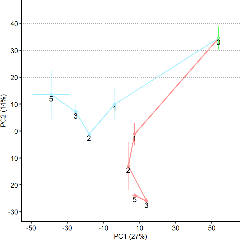
5.1.2 Figure 5B
Diet modulates expression of functionally distinct gene classes. Midguts of flies fed HY diet show higher expression of genes with digestive functions, while HS diet involves mainly genes attributed to stress response and growth. X-axis represents the statistical significance of the gene ontology (GO) categories (y-axis) after adjustment for multiple testing. Size of the dot is proportional to number of genes in the given GO category
tab_GO_results =
d[["5B"]]%>%
mutate_if(is.character,as.factor)%>%
mutate(Padj=-log(p.value,10),
Term = str_to_sentence(Term))%>%
as.data.frame()
tab_GO_results$Term <- factor(tab_GO_results$Term, levels = tab_GO_results$Term[order(tab_GO_results$Diet, tab_GO_results$Padj, tab_GO_results$Significant)])
#order GO categories based on size of Padj
tab_GO_results$Diet <- factor(tab_GO_results$Diet, levels = c("HY", "HS"))
### Plot
Plot_Fig5B=
ggplot(tab_GO_results, aes(x = Padj, y = Term))+
geom_point(aes(size=Significant,fill=Diet),shape=21) +
facet_grid(Diet~.,scales="free_y",space="free")+
scale_fill_manual(limits=c("HS","HY"),
values=c("#FFB4B4","#C3E6FC"))+
geom_vline(xintercept = 1.3,linetype=3)+
scale_y_discrete("GO categories")+
scale_x_continuous(expression(paste("-P-value adjusted (", log[10],")")),
limits=c(0,31),
breaks=c(0,seq(10,30,by=10)))+
scale_size_continuous("Nbr genes", range =c(1,5) )+
theme(panel.grid.major.y = element_line(colour = grey(0.45), linetype = "dashed", size = 0.2),
panel.background = element_blank(),
axis.title.x = element_text(size=Smallfont,colour="black"),
axis.title.y = element_text(size=Smallfont,colour="black"),
axis.line.x = element_line(colour="black",size=0.75),
axis.line.y = element_line(colour="black",size=0.75),
axis.ticks.x = element_line(size = 0.75),
axis.ticks.y = element_line(size = 0.75),
axis.text.x = element_text(size=Smallfont,colour="black"),
axis.text.y = element_text(size=Smallfont-2,colour="black"),
plot.margin = unit(Margin, "cm"),
legend.direction = "horizontal",
legend.box = "horizontal",
legend.position = "top",
legend.key.height = unit(0.4, "cm"),
legend.key.width= unit(0.6, "cm"),
legend.margin=margin(b=0, unit='cm'),
legend.title = element_text(face="italic",size=Smallfont),
legend.key = element_rect(colour = 'white', fill = "white", linetype='dashed'),
legend.text = element_text(size=Smallfont-2),
legend.background = element_rect(fill=NA),
strip.text.x = element_text(size =Smallfont, colour = "black",face="italic"),
strip.text.y = element_text(size = Smallfont, colour = "black", margin = margin(t = 3, r = 1, b = 3, l = 1)),
strip.background = element_rect(fill=NA, colour="black"),
strip.placement="outside")+
guides(fill=F)
Plot_Fig5B
5.1.3 Figure 5C
Table of genes significantly differently expressed, between HS and HY, as a ratio of HS/HY, representing midgut response to HS and HY diets; additional information on the statistics is found in material and methods; asterisks denote genes significantly different for p-value but not for adjusted p-value
img = readImage("F:/Dropbox/Github/Bonfini_eLife_2021/data/5C.jpg")
gob_imageFig5C = rasterGrob(img)
grid.draw(gob_imageFig5C)
5.1.4 Figure 5D
Cell proliferation is possible on HS diet when genetically induced. Progenitor-specific (EsgTS) overexpression of a constitutively active form of Ras (UAS-RasV12) and of UAS-Tor-DER (EGFR Active), both known proliferative inducers, allows for increased proliferation on HS diet. P-values on top of the chart refer to comparison vs control, P-values at the bottom refer to comparison between HS and HY for each sample. Complete statistical annotation on image can be fund in the manuscript’s figures.
Tab_Ras_PH3_Rev =
d[["5D"]]%>%
mutate_at(vars(ends_with(".L")),~./1000)%>%
mutate_at(vars(!starts_with("Total")),as.factor)%>%
dplyr::rename(PH3_positive_cell=Total.PH3,
Diet=Treatment,
Male_Line=Male.Line)%>%
mutate(Cross=fct_relevel(Cross,"EsgTsXControl","EsgTsX64195", "EsgTsXTorDER" ))
###Stats
##Control
tmp = subset(Tab_Ras_PH3_Rev , Male_Line%in%c("Control"))
mod.gen = fitme(log(PH3_positive_cell+1) ~ Diet + (1 | Repeat),data = tmp)
shapiro.test(residuals(mod.gen))
Shapiro-Wilk normality test
data: residuals(mod.gen)
W = 0.98547, p-value = 0.4099bptest(log(PH3_positive_cell+1) ~ Diet + (1 / Repeat),data = tmp)
studentized Breusch-Pagan test
data: log(PH3_positive_cell + 1) ~ Diet + (1/Repeat)
BP = 0.10949, df = 1, p-value = 0.7407mod.gen1 = fitme(log(PH3_positive_cell+1) ~ 1 + (1 | Repeat),data = tmp)
test = anova(mod.gen, mod.gen1)
Chi2_LRT = 2*(mod.gen$APHLs[["p_v"]]-mod.gen1$APHLs[["p_v"]])
tab_stat = data.frame(Variable = as.character(paste("HS vs HY Control")),
Rep = nlevels(Tab_Ras_PH3_Rev$Repeat),
chi2_LR = round(as.numeric(test$basicLRT$chi2_LR), digits = 2),
intercept = format(mod.gen$fixef[1],digits=3),
estimate = format(mod.gen$fixef[2],digits=3),
df = as.numeric(test$basicLRT$df),
Pvalue = as.numeric(format(pchisq(Chi2_LRT,df=1,lower.tail = F),digits=2)))
tab_stat_Control=tab_stat
##Ras85DV12 (64195)
tmp = subset(Tab_Ras_PH3_Rev , Male_Line%in%c("Ras85DV12"))
mod.gen = fitme(log(PH3_positive_cell+1) ~ Diet + (1 | Repeat),data = tmp)
shapiro.test(residuals(mod.gen))
Shapiro-Wilk normality test
data: residuals(mod.gen)
W = 0.98728, p-value = 0.5179bptest(log(PH3_positive_cell+1) ~ Diet + (1 / Repeat),data = tmp)
studentized Breusch-Pagan test
data: log(PH3_positive_cell + 1) ~ Diet + (1/Repeat)
BP = 0.16649, df = 1, p-value = 0.6832mod.gen1 = fitme(log(PH3_positive_cell+1) ~ 1 + (1 | Repeat),data = tmp)
test = anova(mod.gen, mod.gen1)
Chi2_LRT = 2*(mod.gen$APHLs[["p_v"]]-mod.gen1$APHLs[["p_v"]])
tab_stat = data.frame(Variable = as.character(paste("HS vs HY Ras85DV12")),
Rep = nlevels(Tab_Ras_PH3_Rev$Repeat),
chi2_LR = round(as.numeric(test$basicLRT$chi2_LR), digits = 2),
intercept = format(mod.gen$fixef[1],digits=3),
estimate = format(mod.gen$fixef[2],digits=3),
df = as.numeric(test$basicLRT$df),
Pvalue = as.numeric(format(pchisq(Chi2_LRT,df=1,lower.tail = F),digits=2)))
tab_stat_Ras85DV12=tab_stat
##Ras85DV12_2 (TorDER)
tmp = subset(Tab_Ras_PH3_Rev , Male_Line%in%c("TorDER"))
mod.gen = fitme(log(PH3_positive_cell+1) ~ Diet + (1 | Repeat),data = tmp)
shapiro.test(residuals(mod.gen))
Shapiro-Wilk normality test
data: residuals(mod.gen)
W = 0.96675, p-value = 0.1456bptest(log(PH3_positive_cell+1) ~ Diet + (1 / Repeat),data = tmp)
studentized Breusch-Pagan test
data: log(PH3_positive_cell + 1) ~ Diet + (1/Repeat)
BP = 0.77051, df = 1, p-value = 0.3801mod.gen1 = fitme(log(PH3_positive_cell+1) ~ 1 + (1 | Repeat),data = tmp)
test = anova(mod.gen, mod.gen1)
Chi2_LRT = 2*(mod.gen$APHLs[["p_v"]]-mod.gen1$APHLs[["p_v"]])
tab_stat = data.frame(Variable = as.character(paste("HS vs HY TorDER")),
Rep = nlevels(Tab_Ras_PH3_Rev$Repeat),
chi2_LR = round(as.numeric(test$basicLRT$chi2_LR), digits = 2),
intercept = format(mod.gen$fixef[1],digits=3),
estimate = format(mod.gen$fixef[2],digits=3),
df = as.numeric(test$basicLRT$df),
Pvalue = as.numeric(format(pchisq(Chi2_LRT,df=1,lower.tail = F),digits=2)))
tab_stat_TorDER=tab_stat
tab_stat=rbind(tab_stat_Control, tab_stat_Ras85DV12, tab_stat_TorDER)
tab_stat$padj = as.numeric(format(p.adjust(tab_stat$Pvalue, method = "BH"),digits=2,scientific =F))
tab_stat$sig = ifelse(tab_stat$padj < 0.05 & tab_stat$padj > 0.01, "*",
ifelse(tab_stat$padj < 0.01 & tab_stat$padj > 0.001, "**",
ifelse(tab_stat$padj < 0.001, "***", "")))
tab_stat%>%
kable(col.names = c("Comparison", "Replicates", "Chi2","Intercept","Estimate","df" ,"p-value","p-value adjusted","Signif."),row.names = FALSE) %>%
add_header_above(c("log(PH3_positive_cell+1) ~ Diet + (1 | Repeat)" = 9))%>%
kable_styling(bootstrap_options = c("striped", "hover", "condensed"), full_width = F)| Comparison | Replicates | Chi2 | Intercept | Estimate | df | p-value | p-value adjusted | Signif. |
|---|---|---|---|---|---|---|---|---|
| HS vs HY Control | 5 | 0.00 | 1.22 | -0.0117 | 1 | 0.95 | 0.95 | |
| HS vs HY Ras85DV12 | 5 | 1.39 | 3.87 | 0.0679 | 1 | 0.24 | 0.36 | |
| HS vs HY TorDER | 5 | 2.56 | 3.58 | 0.168 | 1 | 0.11 | 0.33 |
tab_stat_rev_RasPH3=tab_stat
tab_stat_rev_RasPH3$Male_Line= tab_stat_rev_RasPH3$Variable
###Stats HS vs control
tmpd = subset(Tab_Ras_PH3_Rev , Diet%in%c("HS"))
##Ras85DV12
tmp = subset(tmpd , Male_Line%in%c("Control", "Ras85DV12"))
mod.gen = fitme((PH3_positive_cell+1) ~ Male_Line + (1 | Repeat),data = tmp)
shapiro.test(residuals(mod.gen))
Shapiro-Wilk normality test
data: residuals(mod.gen)
W = 0.96712, p-value = 0.01814bptest((PH3_positive_cell+1) ~ Male_Line + (1 / Repeat),data = tmp)
studentized Breusch-Pagan test
data: (PH3_positive_cell + 1) ~ Male_Line + (1/Repeat)
BP = 10.691, df = 1, p-value = 0.001077mod.gen1 = fitme((PH3_positive_cell+1) ~ 1 + (1 | Repeat),data = tmp)
test = anova(mod.gen, mod.gen1)
Chi2_LRT = 2*(mod.gen$APHLs[["p_v"]]-mod.gen1$APHLs[["p_v"]])
tab_stat = data.frame(Variable = as.character(paste("HS Ras85DV12 vs HS Control")),
Rep = nlevels(Tab_Ras_PH3_Rev$Repeat),
chi2_LR = round(as.numeric(test$basicLRT$chi2_LR), digits = 2),
intercept = format(mod.gen$fixef[1],digits=3),
estimate = format(mod.gen$fixef[2],digits=3),
df = as.numeric(test$basicLRT$df),
Pvalue = as.numeric(format(pchisq(Chi2_LRT,df=1,lower.tail = F),digits=2)))
tab_stat_HS_Ras85DV12=tab_stat
##TorDER
tmp = subset(tmpd , Male_Line%in%c("Control", "TorDER"))
mod.gen = fitme(log(PH3_positive_cell+1) ~ Male_Line + (1 | Repeat),data = tmp)
shapiro.test(residuals(mod.gen))
Shapiro-Wilk normality test
data: residuals(mod.gen)
W = 0.98961, p-value = 0.8224bptest(log(PH3_positive_cell+1) ~ Male_Line + (1 / Repeat),data = tmp)
studentized Breusch-Pagan test
data: log(PH3_positive_cell + 1) ~ Male_Line + (1/Repeat)
BP = 10.017, df = 1, p-value = 0.001551mod.gen1 = fitme(log(PH3_positive_cell+1) ~ 1 + (1 | Repeat),data = tmp)
test = anova(mod.gen, mod.gen1)
Chi2_LRT = 2*(mod.gen$APHLs[["p_v"]]-mod.gen1$APHLs[["p_v"]])
tab_stat = data.frame(Variable = as.character(paste("HS TorDER vs HS Control")),
Rep = nlevels(Tab_Ras_PH3_Rev$Repeat),
chi2_LR = round(as.numeric(test$basicLRT$chi2_LR), digits = 2),
intercept = format(mod.gen$fixef[1],digits=3),
estimate = format(mod.gen$fixef[2],digits=3),
df = as.numeric(test$basicLRT$df),
Pvalue = as.numeric(format(pchisq(Chi2_LRT,df=1,lower.tail = F),digits=2)))
tab_stat_HS_TorDER=tab_stat
#Table
tab_stat=rbind(tab_stat_HS_Ras85DV12, tab_stat_HS_TorDER)
tab_stat$padj = as.numeric(format(p.adjust(tab_stat$Pvalue, method = "BH"),digits=2,scientific =F))
tab_stat$sig = ifelse(tab_stat$padj < 0.05 & tab_stat$padj > 0.01, "*",
ifelse(tab_stat$padj < 0.01 & tab_stat$padj > 0.001, "**",
ifelse(tab_stat$padj < 0.001, "***", "")))
tab_stat%>%
kable(col.names = c("Comparison", "Replicates", "Chi2","Intercept","Estimate","df" ,"p-value","p-value adjusted","Signif."),row.names = FALSE) %>%
add_header_above(c("log(PH3_positive_cell+1) ~ Genotype + (1 | Repeat)" = 9))%>%
kable_styling(bootstrap_options = c("striped", "hover", "condensed"), full_width = F)| Comparison | Replicates | Chi2 | Intercept | Estimate | df | p-value | p-value adjusted | Signif. |
|---|---|---|---|---|---|---|---|---|
| HS Ras85DV12 vs HS Control | 5 | 138.73 | 6.28 | 45.3 | 1 | 0 | 0 | *** |
| HS TorDER vs HS Control | 5 | 71.82 | 1.23 | 2.46 | 1 | 0 | 0 | *** |
tab_stat_rev_RasPH3_HS=tab_stat
tab_stat_rev_RasPH3_HS$Male_Line= tab_stat_rev_RasPH3_HS$Variable
###Stats HY vs control
tmpd = subset(Tab_Ras_PH3_Rev , Diet%in%c("HY"))
##Ras85DV12
tmp = subset(tmpd , Male_Line%in%c("Control", "Ras85DV12"))
mod.gen = fitme((PH3_positive_cell+1) ~ Male_Line + (1 | Repeat),data = tmp)
shapiro.test(residuals(mod.gen))
Shapiro-Wilk normality test
data: residuals(mod.gen)
W = 0.96149, p-value = 0.009738bptest((PH3_positive_cell+1) ~ Male_Line + (1 / Repeat),data = tmp)
studentized Breusch-Pagan test
data: (PH3_positive_cell + 1) ~ Male_Line + (1/Repeat)
BP = 13.223, df = 1, p-value = 0.0002765mod.gen1 = fitme((PH3_positive_cell+1) ~ 1 + (1 | Repeat),data = tmp)
test = anova(mod.gen, mod.gen1)
Chi2_LRT = 2*(mod.gen$APHLs[["p_v"]]-mod.gen1$APHLs[["p_v"]])
tab_stat = data.frame(Variable = as.character(paste("HY Ras85DV12 vs HY Control")),
Rep = nlevels(Tab_Ras_PH3_Rev$Repeat),
chi2_LR = round(as.numeric(test$basicLRT$chi2_LR), digits = 2),
intercept = format(mod.gen$fixef[1],digits=3),
estimate = format(mod.gen$fixef[2],digits=3),
df = as.numeric(test$basicLRT$df),
Pvalue = as.numeric(format(pchisq(Chi2_LRT,df=1,lower.tail = F),digits=2)))
tab_stat_HY_Ras85DV12=tab_stat
##TorDER
tmp = subset(tmpd , Male_Line%in%c("Control", "TorDER"))
mod.gen = fitme(log(PH3_positive_cell+1) ~ Male_Line + (1 | Repeat),data = tmp)
shapiro.test(residuals(mod.gen))
Shapiro-Wilk normality test
data: residuals(mod.gen)
W = 0.9602, p-value = 0.02268bptest(log(PH3_positive_cell+1) ~ Male_Line + (1 / Repeat),data = tmp)
studentized Breusch-Pagan test
data: log(PH3_positive_cell + 1) ~ Male_Line + (1/Repeat)
BP = 13.229, df = 1, p-value = 0.0002757mod.gen1 = fitme(log(PH3_positive_cell+1) ~ 1 + (1 | Repeat),data = tmp)
test = anova(mod.gen, mod.gen1)
Chi2_LRT = 2*(mod.gen$APHLs[["p_v"]]-mod.gen1$APHLs[["p_v"]])
tab_stat = data.frame(Variable = as.character(paste("HY TorDER vs HY Control")),
Rep = nlevels(Tab_Ras_PH3_Rev$Repeat),
chi2_LR = round(as.numeric(test$basicLRT$chi2_LR), digits = 2),
intercept = format(mod.gen$fixef[1],digits=3),
estimate = format(mod.gen$fixef[2],digits=3),
df = as.numeric(test$basicLRT$df),
Pvalue = as.numeric(format(pchisq(Chi2_LRT,df=1,lower.tail = F),digits=2)))
tab_stat_HY_TorDER=tab_stat
#Table
tab_stat=rbind(tab_stat_HY_Ras85DV12, tab_stat_HY_TorDER)
tab_stat$padj = as.numeric(format(p.adjust(tab_stat$Pvalue, method = "BH"),digits=2,scientific =F))
tab_stat$sig = ifelse(tab_stat$padj < 0.05 & tab_stat$padj > 0.01, "*",
ifelse(tab_stat$padj < 0.01 & tab_stat$padj > 0.001, "**",
ifelse(tab_stat$padj < 0.001, "***", "")))
tab_stat%>%
kable(col.names = c("Comparison", "Replicates", "Chi2","Intercept","Estimate","df" ,"p-value","p-value adjusted","Signif."),row.names = FALSE) %>%
add_header_above(c("log(PH3_positive_cell+1) ~ Genotype + (1 | Repeat)" = 9))%>%
kable_styling(bootstrap_options = c("striped", "hover", "condensed"), full_width = F)| Comparison | Replicates | Chi2 | Intercept | Estimate | df | p-value | p-value adjusted | Signif. |
|---|---|---|---|---|---|---|---|---|
| HY Ras85DV12 vs HY Control | 5 | 141.81 | 5.89 | 47.7 | 1 | 0 | 0 | *** |
| HY TorDER vs HY Control | 5 | 102.66 | 1.2 | 2.67 | 1 | 0 | 0 | *** |
tab_stat_rev_RasPH3_HY=tab_stat
tab_stat_rev_RasPH3_HY$Male_Line= tab_stat_rev_RasPH3_HY$Variable
#Samplesize
Sample_size=
Tab_Ras_PH3_Rev%>%
group_by(Male_Line,Diet)%>%
summarise(Sample_size=n())
### Plot
Tab_Ras_PH3_Rev$Male_Line = factor(Tab_Ras_PH3_Rev$Male_Line, labels = c(expression(italic(paste("Control"))), expression(italic(paste("Ra",s^{V12},sep=""))), expression(italic(paste("Tor-DER")))))
Sample_size$Male_Line = factor(Sample_size$Male_Line, labels = c(expression(italic(paste("Control"))), expression(italic(paste("Ra",s^{V12},sep=""))), expression(italic(paste("Tor-DER")))))
tab_stat_rev_RasPH3$Male_Line = factor(tab_stat_rev_RasPH3$Male_Line, labels = c(expression(italic(paste("Control"))), expression(italic(paste("Ra",s^{V12},sep=""))), expression(italic(paste("Tor-DER")))))
tab_stat_rev_RasPH3_HS$Male_Line = factor(tab_stat_rev_RasPH3_HS$Male_Line, labels = c(expression(italic(paste("Ra",s^{V12},sep=""))), expression(italic(paste("Tor-DER")))))
tab_stat_rev_RasPH3_HY$Male_Line = factor(tab_stat_rev_RasPH3_HY$Male_Line, labels = c(expression(italic(paste("Ra",s^{V12},sep=""))), expression(italic(paste("Tor-DER")))))
#Annotation in the plot
ann_textHS <-data.frame(Male_Line = "Control", anot = "Vs Ctrl HS")
ann_textHS$Male_Line = factor(ann_textHS$Male_Line, labels = c(expression(italic(paste("Control")))))
ann_textHY <-data.frame(Male_Line = "Control", anot = "Vs Ctrl HY")
ann_textHY$Male_Line = factor(ann_textHY$Male_Line, labels = c(expression(italic(paste("Control")))))
ann_text <-data.frame(Male_Line = "Ras85DV12", anot = "HS vs HY")
ann_text$Male_Line = factor(ann_text$Male_Line, labels = c(expression(italic(paste("Ra",s^{V12},sep="")))))
#Plot
Limits = c("HS","HY")
Plot_Fig5D=
ggplot(Tab_Ras_PH3_Rev, aes(x = Diet, y = PH3_positive_cell))+
geom_violin(aes(fill = Diet), draw_quantiles = c(0.25, 0.5, 0.75), colour = "black", size = 0.2,adjust = 0.8) +
geom_dotplot( colour = "black", fill = "white", binaxis = "y", stackdir = "center", binwidth = 3) +
facet_grid(. ~ Male_Line,labeller=label_parsed)+
geom_text(data = Sample_size, mapping = aes(x = Diet, y = -10, label = paste("(",Sample_size,")",sep="")),size=3)+
geom_signif(data = tab_stat_rev_RasPH3, aes(xmin = 1, xmax = 2, annotations = formatC(paste("p=",Pvalue), digits = 2), y_position = 105), textsize = 2.5, vjust = -0.2, manual = TRUE)+
scale_fill_manual(limits=c("HS","HY"),
values=c("#FFB4B4","#C3E6FC"))+
scale_x_discrete("",
limits=Limits,
labels=c("HS","HY"))+
scale_y_continuous(expression(paste("pH3" ^ "+", " cells")),
limits=c(-15,175),
breaks=seq(0,110,by=20))+
stat_summary(fun = mean, geom = "point", size = 3, shape = 18, colour = "black", aes(group = Repeat)) +
stat_summary(fun = mean, geom = "point", size = 2, shape = 18, aes(group = Repeat, colour = Repeat)) +
scale_color_manual(values = palette_mean) +
theme(panel.grid.major.y = element_line(colour = grey(0.45), linetype = "dashed", size = 0.2),
panel.background = element_blank(),
axis.title.x = element_text(size=Smallfont,colour="black"),
axis.title.y = element_text(size=Smallfont,colour="black", margin = margin(t = 0, r = 0, b = 0, l = 0) ),
axis.line.x = element_line(colour="black",size=0.75),
axis.line.y = element_line(colour="black",size=0.75),
axis.ticks.x = element_line(size = 0.75),
axis.ticks.y = element_line(size = 0.75),
axis.text.x = element_text(size=Smallfont,colour="black"),
axis.text.y = element_text(size=Smallfont,colour="black"),
plot.margin = unit(Margin, "cm"),
legend.direction = "vertical",
legend.box = "horizontal",
legend.position = "none",
legend.key.height = unit(0.4, "cm"),
legend.key.width= unit(0.6, "cm"),
legend.title = element_text(face="italic",size=Smallfont),
legend.key = element_rect(colour = 'white', fill = "white", linetype='dashed'),
legend.text = element_text(size=SuperSmallfont),
legend.background = element_rect(fill=NA),
strip.text = element_text(size =Smallfont-2, colour = "black",face="italic", margin = margin(t = 2, r = 1, b = 2, l = 1)),
strip.background = element_rect(fill=NA, colour="black"),
strip.placement="outside")
Plot_Fig5D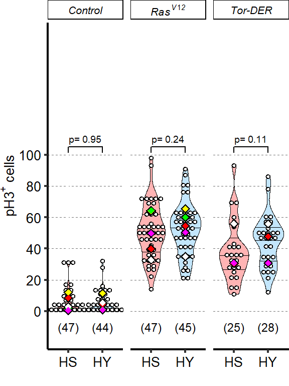
5.1.5 Figure 5E
Enterocyte specific over expression (MyoTS) of UAS-upd3-OE and UAS-spi-SEC elicit increased proliferation, strongly only on HY diet, and weakly on HS with UAS-upd3-OE. P-values on top of the chart refer to comparisons with the control, p-values at the bottom refer to comparison between HS and HY for each sample. Flies were 9 days old when dissected. Complete statistical annotation on image can be fund in the manuscript’s figures.
tab_Myo_PH3_Rev =
d[["5E"]]%>%
mutate_at(vars(ends_with(".L")),~./1000)%>%
mutate_at(vars(!starts_with("Total")),as.factor)%>%
dplyr::rename(PH3_positive_cell=Total.PH3,
Diet=Treatment,
Male_Line=Male.Line)
###Stats HS vs HY
##Control
tmp = subset(tab_Myo_PH3_Rev, Male_Line%in%c("Control"))
mod.gen = fitme(log(PH3_positive_cell+1) ~ Diet + (1 | Repeat),data = tmp)
shapiro.test(residuals(mod.gen))
Shapiro-Wilk normality test
data: residuals(mod.gen)
W = 0.94719, p-value = 0.04711bptest(log(PH3_positive_cell+1) ~ Diet + (1 / Repeat),data = tmp)
studentized Breusch-Pagan test
data: log(PH3_positive_cell + 1) ~ Diet + (1/Repeat)
BP = 2.986, df = 1, p-value = 0.08399mod.gen1 = fitme(log(PH3_positive_cell+1) ~ 1 + (1 | Repeat),data = tmp)
test = anova(mod.gen, mod.gen1)
Chi2_LRT = 2*(mod.gen$APHLs[["p_v"]]-mod.gen1$APHLs[["p_v"]])
tab_stat = data.frame(Comparison = as.character(paste("Control HS vs HY")),
Rep = nlevels(tab_Myo_PH3_Rev$Repeat),
chi2_LR = round(as.numeric(test$basicLRT$chi2_LR), digits = 2),
intercept = format(mod.gen$fixef[1],digits=3),
estimate = format(mod.gen$fixef[2],digits=3),
df = as.numeric(test$basicLRT$df),
Pvalue = as.numeric(format(pchisq(Chi2_LRT,df=1,lower.tail = F),digits=2)))
tab_stat_Control=tab_stat
tab_stat_Control$Male_Line = "Control"
##spi-sec
tmp = subset(tab_Myo_PH3_Rev , Male_Line%in%c("spi-SEC"))
mod.gen = fitme(log(PH3_positive_cell+1) ~ Diet + (1 | Repeat),data = tmp)
shapiro.test(residuals(mod.gen))
Shapiro-Wilk normality test
data: residuals(mod.gen)
W = 0.98552, p-value = 0.8119bptest(log(PH3_positive_cell+1) ~ Diet + (1 / Repeat),data = tmp)
studentized Breusch-Pagan test
data: log(PH3_positive_cell + 1) ~ Diet + (1/Repeat)
BP = 0.079412, df = 1, p-value = 0.7781mod.gen1 = fitme(log(PH3_positive_cell+1) ~ 1 + (1 | Repeat),data = tmp)
test = anova(mod.gen, mod.gen1)
Chi2_LRT = 2*(mod.gen$APHLs[["p_v"]]-mod.gen1$APHLs[["p_v"]])
tab_stat = data.frame(Comparison = as.character(paste("spi-SEC HS vs HY")),
Rep = nlevels(tmp$Repeat),
chi2_LR = round(as.numeric(test$basicLRT$chi2_LR), digits = 2),
intercept = format(mod.gen$fixef[1],digits=3),
estimate = format(mod.gen$fixef[2],digits=3),
df = as.numeric(test$basicLRT$df),
Pvalue = as.numeric(format(pchisq(Chi2_LRT,df=1,lower.tail = F),digits=2)))
tab_stat_spi_sec=tab_stat
tab_stat_spi_sec$Male_Line = "spi-SEC"
##upd3-OE
tmp = subset(tab_Myo_PH3_Rev , Male_Line%in%c("upd3-OE"))
mod.gen = fitme(log(PH3_positive_cell+1) ~ Diet + (1 | Repeat),data = tmp)
shapiro.test(residuals(mod.gen))
Shapiro-Wilk normality test
data: residuals(mod.gen)
W = 0.98739, p-value = 0.8533bptest(log(PH3_positive_cell+1) ~ Diet + (1 / Repeat),data = tmp)
studentized Breusch-Pagan test
data: log(PH3_positive_cell + 1) ~ Diet + (1/Repeat)
BP = 1.9695, df = 1, p-value = 0.1605mod.gen1 = fitme(log(PH3_positive_cell+1) ~ 1 + (1 | Repeat),data = tmp)
test = anova(mod.gen, mod.gen1)
Chi2_LRT = 2*(mod.gen$APHLs[["p_v"]]-mod.gen1$APHLs[["p_v"]])
tab_stat = data.frame(Comparison = as.character(paste("upd3-OE HS vs HY")),
Rep = nlevels(tmp$Repeat),
chi2_LR = round(as.numeric(test$basicLRT$chi2_LR), digits = 2),
intercept = format(mod.gen$fixef[1],digits=3),
estimate = format(mod.gen$fixef[2],digits=3),
df = as.numeric(test$basicLRT$df),
Pvalue = as.numeric(format(pchisq(Chi2_LRT,df=1,lower.tail = F),digits=2)))
tab_stat_upd3_OE=tab_stat
tab_stat_upd3_OE$Male_Line = "upd3-OE"
tab_stat=rbind(tab_stat_Control,tab_stat_spi_sec, tab_stat_upd3_OE)
tab_stat$padj = as.numeric(format(p.adjust(tab_stat$Pvalue, method = "BH"),digits=2,scientific =F))
tab_stat$sig = ifelse(tab_stat$padj < 0.05 & tab_stat$padj > 0.01, "*",
ifelse(tab_stat$padj < 0.01 & tab_stat$padj > 0.001, "**",
ifelse(tab_stat$padj < 0.001, "***", "")))
tab_stat%>%
kable(col.names = c("Comparison", "Replicates", "Chi2","Intercept","Estimate","df" ,"p-value", "Genotype Male_line" ,"p-value adjusted","Signif."),row.names = FALSE) %>%
add_header_above(c("log(PH3_positive_cell+1) ~ Diet + (1 | Repeat)" = 10))%>%
kable_styling(bootstrap_options = c("striped", "hover", "condensed"), full_width = F)| Comparison | Replicates | Chi2 | Intercept | Estimate | df | p-value | Genotype Male_line | p-value adjusted | Signif. |
|---|---|---|---|---|---|---|---|---|---|
| Control HS vs HY | 3 | 0.66 | 2.34 | 0.161 | 1 | 4.2e-01 | Control | 4.2e-01 | |
| spi-SEC HS vs HY | 3 | 21.14 | 2.1 | 1.2 | 1 | 4.3e-06 | spi-SEC | 6.5e-06 | *** |
| upd3-OE HS vs HY | 3 | 77.92 | 3.18 | 1.22 | 1 | 0.0e+00 | upd3-OE | 0.0e+00 | *** |
tab_stat_rev_MyoPH3=tab_stat
###Stats HS vs control
tmpd = subset(tab_Myo_PH3_Rev , Diet%in%c("HS"))
##spi-sec
tmp = subset(tmpd , Male_Line%in%c("Control", "spi-SEC"))
mod.gen = fitme(log(PH3_positive_cell+1) ~ Male_Line + (1 | Repeat),data = tmp)
shapiro.test(residuals(mod.gen))
Shapiro-Wilk normality test
data: residuals(mod.gen)
W = 0.96085, p-value = 0.14bptest(log(PH3_positive_cell+1) ~ Male_Line + (1 / Repeat),data = tmp)
studentized Breusch-Pagan test
data: log(PH3_positive_cell + 1) ~ Male_Line + (1/Repeat)
BP = 0.14417, df = 1, p-value = 0.7042mod.gen1 = fitme(log(PH3_positive_cell+1) ~ 1 + (1 | Repeat),data = tmp)
test = anova(mod.gen, mod.gen1)
Chi2_LRT = 2*(mod.gen$APHLs[["p_v"]]-mod.gen1$APHLs[["p_v"]])
tab_stat = data.frame(Comparison = as.character(paste("Control vs spi-SEC (HS)")),
Rep = nlevels(tmp$Repeat),
chi2_LR = round(as.numeric(test$basicLRT$chi2_LR), digits = 2),
intercept = format(mod.gen$fixef[1],digits=3),
estimate = format(mod.gen$fixef[2],digits=3),
df = as.numeric(test$basicLRT$df),
Pvalue = as.numeric(format(pchisq(Chi2_LRT,df=1,lower.tail = F),digits=2)))
tab_stat_HS_spi_sec=tab_stat
tab_stat_HS_spi_sec$Male_Line = "spi-SEC"
##upd3-OE
tmp = subset(tmpd , Male_Line%in%c("Control", "upd3-OE"))
mod.gen = fitme(log(PH3_positive_cell+1) ~ Male_Line + (1 | Repeat),data = tmp)
shapiro.test(residuals(mod.gen))
Shapiro-Wilk normality test
data: residuals(mod.gen)
W = 0.93704, p-value = 0.01251bptest(log(PH3_positive_cell+1) ~ Male_Line + (1 / Repeat),data = tmp)
studentized Breusch-Pagan test
data: log(PH3_positive_cell + 1) ~ Male_Line + (1/Repeat)
BP = 4.4353, df = 1, p-value = 0.0352mod.gen1 = fitme(log(PH3_positive_cell+1) ~ 1 + (1 | Repeat),data = tmp)
test = anova(mod.gen, mod.gen1)
Chi2_LRT = 2*(mod.gen$APHLs[["p_v"]]-mod.gen1$APHLs[["p_v"]])
tab_stat = data.frame(Comparison = as.character(paste("Control vs upd3-OE (HS)")),
Rep = nlevels(tmp$Repeat),
chi2_LR = round(as.numeric(test$basicLRT$chi2_LR), digits = 2),
intercept = format(mod.gen$fixef[1],digits=3),
estimate = format(mod.gen$fixef[2],digits=3),
df = as.numeric(test$basicLRT$df),
Pvalue = as.numeric(format(pchisq(Chi2_LRT,df=1,lower.tail = F),digits=2)))
tab_stat_HS_upd3_OE=tab_stat
tab_stat_HS_upd3_OE$Male_Line = "upd3-OE"
#Table
tab_stat=rbind(tab_stat_HS_spi_sec, tab_stat_HS_upd3_OE)
tab_stat$padj = as.numeric(format(p.adjust(tab_stat$Pvalue, method = "BH"),digits=2,scientific =F))
tab_stat$sig = ifelse(tab_stat$padj < 0.05 & tab_stat$padj > 0.01, "*",
ifelse(tab_stat$padj < 0.01 & tab_stat$padj > 0.001, "**",
ifelse(tab_stat$padj < 0.001, "***", "")))
tab_stat%>%
kable(col.names = c("Comparison", "Replicates", "Chi2","Intercept","Estimate","df" ,"p-value","Genotype Male_Line" ,"p-value adjusted","Signif."),row.names = FALSE) %>%
add_header_above(c("log(PH3_positive_cell+1) ~ Genotype + (1 | Repeat)" = 10))%>%
kable_styling(bootstrap_options = c("striped", "hover", "condensed"), full_width = F)| Comparison | Replicates | Chi2 | Intercept | Estimate | df | p-value | Genotype Male_Line | p-value adjusted | Signif. |
|---|---|---|---|---|---|---|---|---|---|
| Control vs spi-SEC (HS) | 3 | 1.42 | 2.38 | -0.295 | 1 | 2.3e-01 | spi-SEC | 2.3e-01 | |
| Control vs upd3-OE (HS) | 3 | 18.54 | 2.34 | 0.836 | 1 | 1.7e-05 | upd3-OE | 3.4e-05 | *** |
tab_stat_rev_MyoPH3_HS=tab_stat
###Stats HY vs control
tmpd = subset(tab_Myo_PH3_Rev , Diet%in%c("HY"))
##spi-sec
tmp = subset(tmpd , Male_Line%in%c("Control", "spi-SEC"))
mod.gen = fitme(log(PH3_positive_cell+1) ~ Male_Line + (1 | Repeat),data = tmp)
shapiro.test(residuals(mod.gen))
Shapiro-Wilk normality test
data: residuals(mod.gen)
W = 0.96573, p-value = 0.1812bptest(log(PH3_positive_cell+1) ~ Male_Line + (1 / Repeat),data = tmp)
studentized Breusch-Pagan test
data: log(PH3_positive_cell + 1) ~ Male_Line + (1/Repeat)
BP = 6.342, df = 1, p-value = 0.01179mod.gen1 = fitme(log(PH3_positive_cell+1) ~ 1 + (1 | Repeat),data = tmp)
test = anova(mod.gen, mod.gen1)
Chi2_LRT = 2*(mod.gen$APHLs[["p_v"]]-mod.gen1$APHLs[["p_v"]])
tab_stat = data.frame(Comparison = as.character(paste("Control vs spi-SEC (HY)")),
Rep = nlevels(tmp$Repeat),
chi2_LR = round(as.numeric(test$basicLRT$chi2_LR), digits = 2),
intercept = format(mod.gen$fixef[1],digits=3),
estimate = format(mod.gen$fixef[2],digits=3),
df = as.numeric(test$basicLRT$df),
Pvalue = as.numeric(format(pchisq(Chi2_LRT,df=1,lower.tail = F),digits=2)))
tab_stat_HY_spi_sec=tab_stat
tab_stat_HY_spi_sec$Male_Line = "spi-SEC"
##upd3-OE
tmp = subset(tmpd , Male_Line%in%c("Control", "upd3-OE"))
mod.gen = fitme(log(PH3_positive_cell+1) ~ Male_Line + (1 | Repeat),data = tmp)
shapiro.test(residuals(mod.gen))
Shapiro-Wilk normality test
data: residuals(mod.gen)
W = 0.9556, p-value = 0.07199bptest(log(PH3_positive_cell+1) ~ Male_Line + (1 / Repeat),data = tmp)
studentized Breusch-Pagan test
data: log(PH3_positive_cell + 1) ~ Male_Line + (1/Repeat)
BP = 4.3033, df = 1, p-value = 0.03804mod.gen1 = fitme(log(PH3_positive_cell+1) ~ 1 + (1 | Repeat),data = tmp)
test = anova(mod.gen, mod.gen1)
Chi2_LRT = 2*(mod.gen$APHLs[["p_v"]]-mod.gen1$APHLs[["p_v"]])
tab_stat = data.frame(Comparison = as.character(paste("Control vs upd3-OE (HY)")),
Rep = nlevels(tmp$Repeat),
chi2_LR = round(as.numeric(test$basicLRT$chi2_LR), digits = 2),
intercept = format(mod.gen$fixef[1],digits=3),
estimate = format(mod.gen$fixef[2],digits=3),
df = as.numeric(test$basicLRT$df),
Pvalue = as.numeric(format(pchisq(Chi2_LRT,df=1,lower.tail = F),digits=2)))
tab_stat_HY_upd3_OE=tab_stat
tab_stat_HY_upd3_OE$Male_Line = "upd3-OE"
#Table
tab_stat=rbind(tab_stat_HY_spi_sec, tab_stat_HY_upd3_OE)
tab_stat$padj = as.numeric(format(p.adjust(tab_stat$Pvalue, method = "BH"),digits=2,scientific =F))
tab_stat$sig = ifelse(tab_stat$padj < 0.05 & tab_stat$padj > 0.01, "*",
ifelse(tab_stat$padj < 0.01 & tab_stat$padj > 0.001, "**",
ifelse(tab_stat$padj < 0.001, "***", "")))
tab_stat%>%
kable(col.names = c("Comparison", "Replicates", "Chi2","Intercept","Estimate","df" ,"p-value", "Genotype Male_Line" ,"p-value adjusted","Signif."),row.names = FALSE) %>%
add_header_above(c("log(PH3_positive_cell+1) ~ Genotype + (1 | Repeat)" = 10))%>%
kable_styling(bootstrap_options = c("striped", "hover", "condensed"), full_width = F)| Comparison | Replicates | Chi2 | Intercept | Estimate | df | p-value | Genotype Male_Line | p-value adjusted | Signif. |
|---|---|---|---|---|---|---|---|---|---|
| Control vs spi-SEC (HY) | 3 | 13.05 | 2.5 | 0.774 | 1 | 3e-04 | spi-SEC | 3e-04 | *** |
| Control vs upd3-OE (HY) | 3 | 112.62 | 2.41 | 1.98 | 1 | 0e+00 | upd3-OE | 0e+00 | *** |
tab_stat_rev_MyoPH3_HY=tab_stat
Sample_size=
tab_Myo_PH3_Rev%>%
group_by(Male_Line,Diet)%>%
summarise(Sample_size=n())
#Annotation in the plot
ann_textHS <-data.frame(Male_Line = "Control", anot = "Vs Ctrl HS")
ann_textHY <-data.frame(Male_Line = "Control", anot = "Vs Ctrl HY")
ann_text <-data.frame(Male_Line = "spi-SEC", anot = "HS vs HY")
### Plot
Limits = c("HS","HY")
Plot_Fig5E=
ggplot(tab_Myo_PH3_Rev, aes(x = Diet, y = PH3_positive_cell))+
geom_violin(aes(fill = Diet), draw_quantiles = c(0.25, 0.5, 0.75), colour = "black", size = 0.2,adjust = 0.8) +
geom_dotplot( colour = "black", fill = "white", binaxis = "y", stackdir = "center", binwidth = 3) +
geom_text(data = Sample_size, mapping = aes(x = Diet, y = -10, label = paste("(",Sample_size,")",sep="")),size=3)+
geom_signif(data = tab_stat_rev_MyoPH3, aes(xmin = 1, xmax = 2, annotations = formatC(paste("p=",Pvalue), digits = 2), y_position = 135), textsize = 2.5, vjust = -0.2, manual = TRUE)+
facet_grid(. ~ Male_Line)+
scale_fill_manual(limits=c("HS","HY"),
values=c("#FFB4B4","#C3E6FC"))+
scale_x_discrete("",
limits=Limits,
labels=c("HS","HY"))+
scale_y_continuous(expression(paste("pH3" ^ "+", " cells")),
limits=c(-15,225),
breaks=seq(0,130,by=20))+
stat_summary(fun = mean, geom = "point", size = 3, shape = 18, colour = "black", aes(group = Repeat)) +
stat_summary(fun = mean, geom = "point", size = 2, shape = 18, aes(group = Repeat, colour = Repeat)) +
scale_color_manual(values = palette_mean) +
theme(panel.grid.major.y = element_line(colour = grey(0.45), linetype = "dashed", size = 0.2),
panel.background = element_blank(),
axis.title.x = element_text(size=Smallfont,colour="black"),
axis.title.y = element_text(size=Smallfont,colour="black", margin = margin(t = 0, r = 0, b = 0, l = 0) ),
axis.line.x = element_line(colour="black",size=0.75),
axis.line.y = element_line(colour="black",size=0.75),
axis.ticks.x = element_line(size = 0.75),
axis.ticks.y = element_line(size = 0.75),
axis.text.x = element_text(size=Smallfont,colour="black"),
axis.text.y = element_text(size=Smallfont,colour="black"),
plot.margin = unit(Margin, "cm"),
legend.direction = "vertical",
legend.box = "horizontal",
legend.position = "none",
legend.key.height = unit(0.4, "cm"),
legend.key.width= unit(0.6, "cm"),
legend.title = element_text(face="italic",size=Smallfont),
legend.key = element_rect(colour = 'white', fill = "white", linetype='dashed'),
legend.text = element_text(size=SuperSmallfont),
legend.background = element_rect(fill=NA),
strip.text.x = element_text(size = xSmallfont, colour = "black", angle=0, face = "italic", margin = margin(t = 2, r = 0, b = 2, l = 0)),
strip.text.y = element_text(size = xSmallfont, colour = "black", angle=0, face = "italic", margin = margin(t = 2, r = 0, b = 2, l = 0)),
strip.background = element_rect(fill=NA, colour="black"),
strip.placement="outside")
Plot_Fig5E
5.1.6 Figure 5F-G
General translation is lower on HS than HY, shown by puromycin incorporation assay. Images show lower incorporation on HS (F, F’, top row) than HY (G, G’, bottom row) in region 4 of the midgut.Complete graphical annotation can be found in manuscript figures
img = readImage("F:/Dropbox/Github/Bonfini_eLife_2021/data/5F.jpg")
gob_imageFig5F = rasterGrob(img)
grid.draw(gob_imageFig5F)
img = readImage("F:/Dropbox/Github/Bonfini_eLife_2021/data/5F'.jpg")
gob_imageFig5F2 = rasterGrob(img)
grid.draw(gob_imageFig5F2)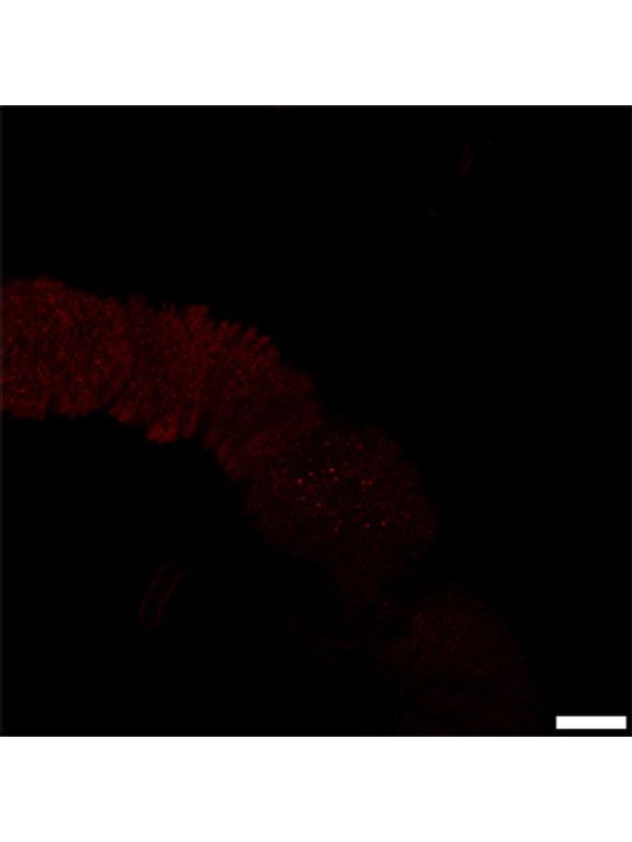
img = readImage("F:/Dropbox/Github/Bonfini_eLife_2021/data/5G.jpg")
gob_imageFig5G = rasterGrob(img)
grid.draw(gob_imageFig5G)
img = readImage("F:/Dropbox/Github/Bonfini_eLife_2021/data/5G'.jpg")
gob_imageFig5G2 = rasterGrob(img)
grid.draw(gob_imageFig5G2)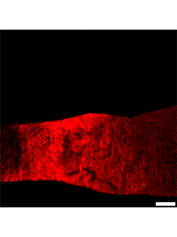
5.1.7 Figure 5H
Quantification of mean pixel intensity of puromycin stain.
Length_Puromycin =
d[["5H"]]%>%
mutate_if(is.character,as.factor)%>%
mutate_if(is.integer,as.factor)%>%
dplyr::rename(Puromycin_int=Mean)
Sample_size=
Length_Puromycin%>%
group_by(Diet)%>%
summarise(Sample_size=n())
###Stats
mod.gen = fitme(log(Puromycin_int) ~ Diet + (1 | Repeat),data = Length_Puromycin)
shapiro.test(residuals(mod.gen))
Shapiro-Wilk normality test
data: residuals(mod.gen)
W = 0.95472, p-value = 0.1274bptest(log(Puromycin_int) ~ Diet + (1 / Repeat),data = Length_Puromycin)
studentized Breusch-Pagan test
data: log(Puromycin_int) ~ Diet + (1/Repeat)
BP = 4.3831, df = 1, p-value = 0.0363mod.gen1 = fitme(log(Puromycin_int) ~ 1 + (1 | Repeat),data = Length_Puromycin)
test = anova(mod.gen, mod.gen1)
Chi2_LRT = 2*(mod.gen$APHLs[["p_v"]]-mod.gen1$APHLs[["p_v"]])
tab_stat = data.frame(Variable = as.character(paste("HS vs HY")),
Rep = nlevels(Length_Puromycin$Repeat),
chi2_LR = round(as.numeric(test$basicLRT$chi2_LR), digits = 2),
intercept = format(mod.gen$fixef[1],digits=3),
estimate = format(mod.gen$fixef[2],digits=3),
df = as.numeric(test$basicLRT$df),
Pvalue = as.numeric(format(pchisq(Chi2_LRT,df=1,lower.tail = F),digits=2)))
tab_stat$sig = ifelse(tab_stat$Pvalue < 0.05 & tab_stat$Pvalue > 0.01, "*",
ifelse(tab_stat$Pvalue < 0.01 & tab_stat$Pvalue > 0.001, "**",
ifelse(tab_stat$Pvalue < 0.001, "***", "")))
tab_stat%>%
kable(col.names = c("Comparison", "Replicates", "Chi2","Intercept","Estimate","df" ,"p-value","Signif."),row.names = FALSE) %>% add_header_above(c("log(Puromycin intensity) ~ Diet + (1 | Repeat)" = 8))%>%
kable_styling(bootstrap_options = c("striped", "hover", "condensed"), full_width = F)| Comparison | Replicates | Chi2 | Intercept | Estimate | df | p-value | Signif. |
|---|---|---|---|---|---|---|---|
| HS vs HY | 3 | 17.81 | 1.86 | 0.911 | 1 | 2.4e-05 | *** |
### Plot
Plot_Fig5H=
ggplot(Length_Puromycin, aes(x = Diet, y = Puromycin_int))+
geom_violin(aes(fill = Diet), draw_quantiles = c(0.25, 0.5, 0.75), colour = "black", size = 0.2,adjust = 0.8) +
geom_dotplot( colour = "black", fill = "white", binaxis = "y", stackdir = "center", binwidth = 1) +
geom_text(data = Sample_size, mapping = aes(x = Diet, y = 1, label = paste("(",Sample_size,")",sep="")),size=3)+
geom_signif(annotation = formatC(paste("p=",tab_stat$Pvalue), digits = 2), textsize = 3, y_position = 47, xmin = 1, xmax = 2, tip_length = c(0.02, 0.02), vjust = -0.2)+
scale_fill_manual(limits=c("HS","HY"),
values=c("#FFB4B4","#C3E6FC"))+
scale_x_discrete("",
limits=c("HS","HY"),
labels=c("HS","HY"))+
scale_y_continuous("Mean pixel intensity
puromycin (a.u.)",
limits=c(0,50),
breaks=seq(0,40,by=10))+
stat_summary(fun = mean, geom = "point", size = 3, shape = 18, colour = "black", aes(group = Repeat)) +
stat_summary(fun = mean, geom = "point", size = 2, shape = 18, aes(group = Repeat, colour = Repeat)) +
scale_color_manual(values = palette_mean) +
theme(panel.grid.major.y = element_line(colour = grey(0.45), linetype = "dashed", size = 0.2),
panel.background = element_blank(),
axis.title.x = element_text(size=Smallfont,colour="black"),
axis.title.y = element_text(size=Smallfont,colour="black"),
axis.line.x = element_line(colour="black",size=0.75),
axis.line.y = element_line(colour="black",size=0.75),
axis.ticks.x = element_line(size = 0.75),
axis.ticks.y = element_line(size = 0.75),
axis.text.x = element_text(size=Smallfont,colour="black"),
axis.text.y = element_text(size=Smallfont,colour="black"),
plot.margin = unit(Margin, "cm"),
legend.direction = "vertical",
legend.box = "horizontal",
legend.position = "none",
legend.key.height = unit(0.4, "cm"),
legend.key.width= unit(0.6, "cm"),
legend.title = element_text(face="italic",size=Smallfont),
legend.key = element_rect(colour = 'white', fill = "white", linetype='dashed'),
legend.text = element_text(size=SuperSmallfont),
legend.background = element_rect(fill=NA),
strip.text = element_text(size =Smallfont-2, colour = "black",face="italic", margin = margin(t = 2, r = 0, b = 2, l = 0)),
strip.background = element_rect(fill=NA, colour="black"),
strip.placement="outside")
Plot_Fig5H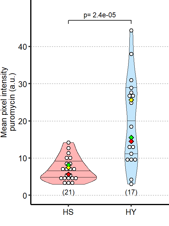
5.1.8 Figure 5I-J
p-eIF2α stain is elevated on HS (I, I’, top row) compared to HY (J, J’, bottom row). Complete graphical annotation can be found in manuscript figures
img = readImage("F:/Dropbox/Github/Bonfini_eLife_2021/data/5I.jpg")
gob_imageFig5I = rasterGrob(img)
grid.draw(gob_imageFig5I)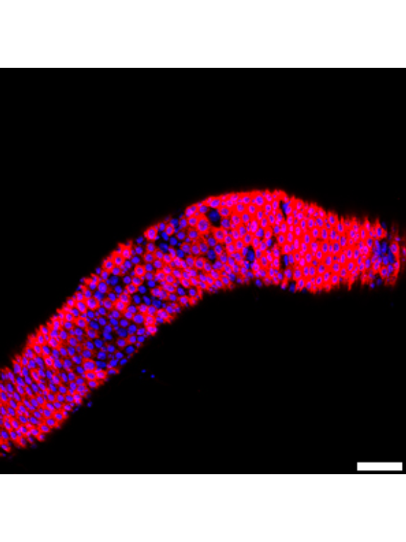
img = readImage("F:/Dropbox/Github/Bonfini_eLife_2021/data/5I'.jpg")
gob_imageFig5I2 = rasterGrob(img)
grid.draw(gob_imageFig5I2)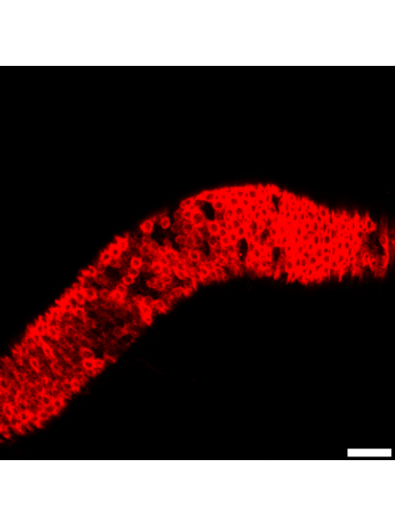
img = readImage("F:/Dropbox/Github/Bonfini_eLife_2021/data/5J.jpg")
gob_imageFig5J = rasterGrob(img)
grid.draw(gob_imageFig5J)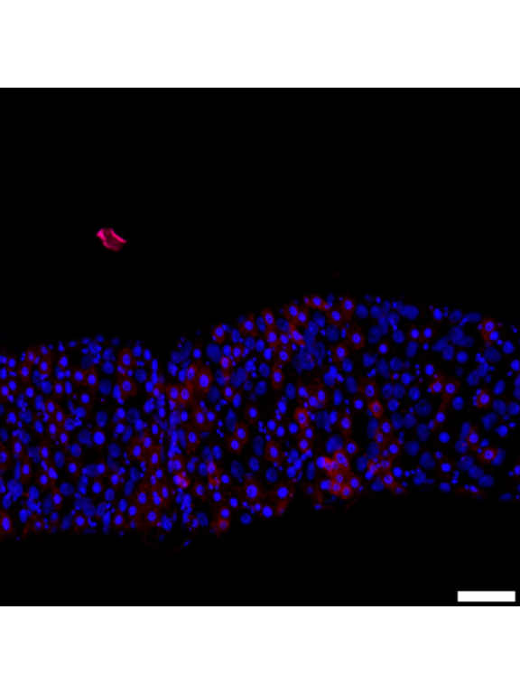
img = readImage("F:/Dropbox/Github/Bonfini_eLife_2021/data/5J'.jpg")
gob_imageFig5J2 = rasterGrob(img)
grid.draw(gob_imageFig5J2)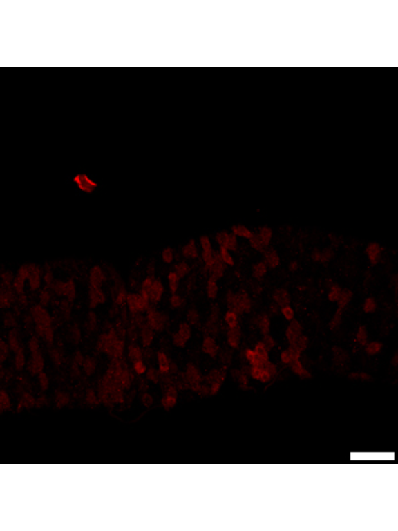
5.1.9 Figure 5K
Quantification of mean pixel intensity of p-eIF2α stain.
Length_EIF2 =
d[["5K"]]%>%
mutate_if(is.character,as.factor)%>%
mutate_if(is.integer,as.factor)%>%
dplyr::rename(EIF2_int=Mean)
Sample_size=
Length_EIF2%>%
group_by(Diet)%>%
summarise(Sample_size=n())
###Stats
mod.gen = fitme(log(EIF2_int) ~ Diet + (1 | Repeat),data = Length_EIF2)
shapiro.test(residuals(mod.gen))
Shapiro-Wilk normality test
data: residuals(mod.gen)
W = 0.88642, p-value = 0.004706bptest(log(EIF2_int) ~ Diet + (1 / Repeat),data = Length_EIF2)
studentized Breusch-Pagan test
data: log(EIF2_int) ~ Diet + (1/Repeat)
BP = 0.097825, df = 1, p-value = 0.7545mod.gen1 = fitme(log(EIF2_int) ~ 1 + (1 | Repeat),data = Length_EIF2)
test = anova(mod.gen, mod.gen1)
Chi2_LRT = 2*(mod.gen$APHLs[["p_v"]]-mod.gen1$APHLs[["p_v"]])
tab_stat = data.frame(Variable = as.character(paste("HS vs HY")),
Rep = nlevels(Length_EIF2$Repeat),
chi2_LR = round(as.numeric(test$basicLRT$chi2_LR), digits = 2),
intercept = format(mod.gen$fixef[1],digits=3),
estimate = format(mod.gen$fixef[2],digits=3),
df = as.numeric(test$basicLRT$df),
Pvalue = as.numeric(format(pchisq(Chi2_LRT,df=1,lower.tail = F),digits=2)))
tab_stat$sig = ifelse(tab_stat$Pvalue < 0.05 & tab_stat$Pvalue > 0.01, "*",
ifelse(tab_stat$Pvalue < 0.01 & tab_stat$Pvalue > 0.001, "**",
ifelse(tab_stat$Pvalue < 0.001, "***", "")))
tab_stat%>%
kable(col.names = c("Comparison", "Replicates", "Chi2","Intercept","Estimate","df" ,"p-value","Signif."),row.names = FALSE) %>% add_header_above(c("log(EIF2 intensity) ~ Diet + (1 | Repeat)" = 8))%>%
kable_styling(bootstrap_options = c("striped", "hover", "condensed"), full_width = F)| Comparison | Replicates | Chi2 | Intercept | Estimate | df | p-value | Signif. |
|---|---|---|---|---|---|---|---|
| HS vs HY | 3 | 15.54 | 4.34 | -0.781 | 1 | 8.1e-05 | *** |
### Plot
Plot_Fig5K=
ggplot(Length_EIF2, aes(x = Diet, y = EIF2_int))+
geom_boxplot(aes(fill = Diet), colour = "black", size = 0.2,outlier.shape = NA) +
geom_dotplot( colour = "black", fill = "white", binaxis = "y", stackdir = "center", binwidth = 3) +
geom_text(data = Sample_size, mapping = aes(x = Diet, y = 3, label = paste("(",Sample_size,")",sep="")),size=3)+
geom_signif(annotation = formatC(paste("p=",tab_stat$Pvalue), digits = 2), textsize = 3, y_position = 135, xmin = 1, xmax = 2, tip_length = c(0.02, 0.02), vjust = -0.2)+
scale_fill_manual(limits=c("HS","HY"),
values=c("#FFB4B4","#C3E6FC"))+
scale_x_discrete("",
limits=c("HS","HY"),
labels=c("HS","HY"))+
scale_y_continuous(expression(paste("Mean pixel intensity p-eIF2",alpha," (a.u.)",sep="")),
limits=c(0,140),
breaks=seq(0,125,by=25))+
stat_summary(fun = mean, geom = "point", size = 3, shape = 18, colour = "black", aes(group = Repeat)) +
stat_summary(fun = mean, geom = "point", size = 2, shape = 18, aes(group = Repeat, colour = Repeat)) +
scale_color_manual(values = palette_mean) +
theme(panel.grid.major.y = element_line(colour = grey(0.45), linetype = "dashed", size = 0.2),
panel.background = element_blank(),
axis.title.x = element_text(size=Smallfont,colour="black"),
axis.title.y = element_text(size=Smallfont,colour="black"),
axis.line.x = element_line(colour="black",size=0.75),
axis.line.y = element_line(colour="black",size=0.75),
axis.ticks.x = element_line(size = 0.75),
axis.ticks.y = element_line(size = 0.75),
axis.text.x = element_text(size=Smallfont,colour="black"),
axis.text.y = element_text(size=Smallfont,colour="black"),
plot.margin = unit(Margin, "cm"),
legend.direction = "vertical",
legend.box = "horizontal",
legend.position = "none",
legend.key.height = unit(0.4, "cm"),
legend.key.width= unit(0.6, "cm"),
legend.title = element_text(face="italic",size=Smallfont),
legend.key = element_rect(colour = 'white', fill = "white", linetype='dashed'),
legend.text = element_text(size=SuperSmallfont),
legend.background = element_rect(fill=NA),
strip.text = element_text(size =Smallfont-2, colour = "black",face="italic"),
strip.background = element_rect(fill=NA, colour="black"),
strip.placement="outside")
Plot_Fig5K
5.1.10 Figure 5L
Re-enabling translation can restore mitosis in midguts shrinking after being shifted from HY to HS diet for 7 days. Blocking translational inhibition with ActTS>Gcn2-IR or ActTS>LK6-IR is sufficient to increase pH3+ cells in midguts of flies on HS diet. However, ActTS>PEK-IR and ActTS>AMPKα-IR had no effect on the number of pH3+ cells. Statistical comparisons are vs control. Full statistical annotation on chart in pubblication
tab_PH3_Translation =
d[["5L"]]%>%
mutate_at(vars(!starts_with("Total")),as.factor)%>%
dplyr::rename(PH3_positive_cell=Total.PH3,
Day_of_treatment=Day)%>%
mutate(Male.Line=fct_relevel(Male.Line,c("Control","Ampk-IR","PEK-IR", "Gcn2-IR", "Lk6-IR")))
Sample_size=
tab_PH3_Translation%>%
group_by(Male.Line)%>%
summarise(Sample_size=n())
###Stats
#Gcn2-IR
tmp = subset(tab_PH3_Translation,!is.na(PH3_positive_cell) & Male.Line%in%c("Control","Gcn2-IR"))
mod.gen = fitme(log(PH3_positive_cell+1) ~ Male.Line + (1 | Repeat),data = tmp)
shapiro.test(residuals(mod.gen))
Shapiro-Wilk normality test
data: residuals(mod.gen)
W = 0.9651, p-value = 0.1908bptest(log(PH3_positive_cell+1) ~ Male.Line + (1 / Repeat),data = tmp)
studentized Breusch-Pagan test
data: log(PH3_positive_cell + 1) ~ Male.Line + (1/Repeat)
BP = 0.68353, df = 1, p-value = 0.4084mod.gen1 = fitme(log(PH3_positive_cell+1) ~ 1 + (1 | Repeat),data = tmp)
test = anova(mod.gen, mod.gen1)
Chi2_LRT_growth = 2*(mod.gen$APHLs[["p_v"]]-mod.gen1$APHLs[["p_v"]])
tab_stat = data.frame(Male.Line = as.character(paste("Gcn2-IR")),
Rep = nlevels(tmp$Repeat),
chi2_LR = round(as.numeric(test$basicLRT$chi2_LR), digits = 2),
intercept = format(mod.gen$fixef[1],digits=3),
estimate = format(mod.gen$fixef[2],digits=3),
df = as.numeric(test$basicLRT$df),
Pvalue = as.numeric(format(pchisq(Chi2_LRT_growth,df=1,lower.tail = F),digits=2)))
tab_stat_GCN=tab_stat
#PEK-IR
tmp = subset(tab_PH3_Translation,!is.na(PH3_positive_cell) & Male.Line%in%c("Control","PEK-IR"))
mod.gen = fitme(log(PH3_positive_cell+1) ~ Male.Line + (1 | Repeat),data = tmp)
shapiro.test(residuals(mod.gen))
Shapiro-Wilk normality test
data: residuals(mod.gen)
W = 0.95637, p-value = 0.1094bptest(log(PH3_positive_cell+1) ~ Male.Line + (1 / Repeat),data = tmp)
studentized Breusch-Pagan test
data: log(PH3_positive_cell + 1) ~ Male.Line + (1/Repeat)
BP = 1.0797, df = 1, p-value = 0.2988mod.gen1 = fitme(log(PH3_positive_cell+1) ~ 1 + (1 | Repeat),data = tmp)
test = anova(mod.gen, mod.gen1)
Chi2_LRT_growth = 2*(mod.gen$APHLs[["p_v"]]-mod.gen1$APHLs[["p_v"]])
tab_stat = data.frame(Male.Line = as.character(paste("PEK-IR")),
Rep = nlevels(tmp$Repeat),
chi2_LR = round(as.numeric(test$basicLRT$chi2_LR), digits = 2),
intercept = format(mod.gen$fixef[1],digits=3),
estimate = format(mod.gen$fixef[2],digits=3),
df = as.numeric(test$basicLRT$df),
Pvalue = as.numeric(format(pchisq(Chi2_LRT_growth,df=1,lower.tail = F),digits=1,scientific=F)))
tab_stat_PEK=tab_stat
#Lk6-IR
tmp = subset(tab_PH3_Translation,!is.na(PH3_positive_cell) & Male.Line%in%c("Control","Lk6-IR"))
mod.gen = fitme(log(PH3_positive_cell+1) ~ Male.Line + (1 | Repeat),data = tmp)
shapiro.test(residuals(mod.gen))
Shapiro-Wilk normality test
data: residuals(mod.gen)
W = 0.97495, p-value = 0.4461bptest(log(PH3_positive_cell+1) ~ Male.Line + (1 / Repeat),data = tmp)
studentized Breusch-Pagan test
data: log(PH3_positive_cell + 1) ~ Male.Line + (1/Repeat)
BP = 0.0018974, df = 1, p-value = 0.9653mod.gen1 = fitme(log(PH3_positive_cell+1) ~ 1 + (1 | Repeat),data = tmp)
test = anova(mod.gen, mod.gen1)
Chi2_LRT_growth = 2*(mod.gen$APHLs[["p_v"]]-mod.gen1$APHLs[["p_v"]])
tab_stat = data.frame(Male.Line = as.character(paste("Lk6-IR")),
Rep = nlevels(tmp$Repeat),
chi2_LR = round(as.numeric(test$basicLRT$chi2_LR), digits = 2),
intercept = format(mod.gen$fixef[1],digits=3),
estimate = format(mod.gen$fixef[2],digits=3),
df = as.numeric(test$basicLRT$df),
Pvalue = as.numeric(format(pchisq(Chi2_LRT_growth,df=1,lower.tail = F),digits=5)))
tab_stat_Lk6=tab_stat
#Ampk-IR
tmp = subset(tab_PH3_Translation,!is.na(PH3_positive_cell) & Male.Line%in%c("Control","Ampk-IR"))
mod.gen = fitme(log(PH3_positive_cell+1) ~ Male.Line + (1 | Repeat),data = tmp)
shapiro.test(residuals(mod.gen))
Shapiro-Wilk normality test
data: residuals(mod.gen)
W = 0.95512, p-value = 0.09866bptest(log(PH3_positive_cell+1) ~ Male.Line + (1 / Repeat),data = tmp)
studentized Breusch-Pagan test
data: log(PH3_positive_cell + 1) ~ Male.Line + (1/Repeat)
BP = 2.3767, df = 1, p-value = 0.1232mod.gen1 = fitme(log(PH3_positive_cell+1) ~ 1 + (1 | Repeat),data = tmp)
test = anova(mod.gen, mod.gen1)
Chi2_LRT_growth = 2*(mod.gen$APHLs[["p_v"]]-mod.gen1$APHLs[["p_v"]])
tab_stat = data.frame(Male.Line = as.character(paste("Ampk-IR")),
Rep = nlevels(tmp$Repeat),
chi2_LR = round(as.numeric(test$basicLRT$chi2_LR), digits = 2),
intercept = format(mod.gen$fixef[1],digits=3),
estimate = format(mod.gen$fixef[2],digits=3),
df = as.numeric(test$basicLRT$df),
Pvalue = as.numeric(format(pchisq(Chi2_LRT_growth,df=1,lower.tail = F),digits=2,scientific=F)))
tab_stat_Ampk=tab_stat
tab_stat=rbind(tab_stat_PEK,tab_stat_Ampk,tab_stat_Lk6,tab_stat_GCN)
tab_stat$padj = as.numeric(format(p.adjust(tab_stat$Pvalue, method = "BH"),digits=2,scientific =T))
tab_stat$sig = ifelse(tab_stat$padj < 0.05 & tab_stat$padj > 0.01, "*",
ifelse(tab_stat$padj < 0.01 & tab_stat$padj > 0.001, "**",
ifelse(tab_stat$padj < 0.001, "***", "")))
tab_stat%>%
kable(col.names = c("Difference in Diet", "Replicates", "Chi2","Intercept","Estimate","df" ,"p-value","p-value adjusted","Signif."),row.names = FALSE) %>%
add_header_above(c("log(PH3_positive_cell+1) ~ Genotype + (1 | Repeat)" = 9))%>%
kable_styling(bootstrap_options = c("striped", "hover", "condensed"), full_width = F)| Difference in Diet | Replicates | Chi2 | Intercept | Estimate | df | p-value | p-value adjusted | Signif. |
|---|---|---|---|---|---|---|---|---|
| PEK-IR | 3 | 2.77 | 1.74 | 0.301 | 1 | 1.0e-01 | 1.3e-01 | |
| Ampk-IR | 3 | 0.40 | 1.76 | 0.13 | 1 | 5.3e-01 | 5.3e-01 | |
| Lk6-IR | 3 | 38.20 | 1.75 | 1.39 | 1 | 0.0e+00 | 0.0e+00 | *** |
| Gcn2-IR | 3 | 23.61 | 1.74 | 0.926 | 1 | 1.2e-06 | 2.4e-06 | *** |
letter_position = aggregate(data=tab_PH3_Translation,PH3_positive_cell ~ Male.Line, max)
tab_stat=left_join(tab_stat,letter_position)
tab_stat5L = tab_stat
### Plot
tab_PH3_Translation$Female.Line = factor(tab_PH3_Translation$Female.Line, labels = c(expression(italic(paste("Ac",t^{TS},">",sep="")))))
z=max(tab_PH3_Translation$PH3_positive_cell, na.rm = TRUE)
Plot_Fig5L=
ggplot(tab_PH3_Translation, aes(x = Male.Line, y = PH3_positive_cell))+
geom_violin(aes(fill = Diet), draw_quantiles = c(0.25, 0.5, 0.75), colour = "black", size = 0.2,adjust = 0.8) +
geom_dotplot( colour = "black", fill = "white", binaxis = "y", stackdir = "center", binwidth = z/40) +
geom_text(data = Sample_size, mapping = aes(x = Male.Line, y = -3, label = paste("(",Sample_size,")",sep="")),size=3)+
facet_grid(.~Female.Line, labeller = label_parsed)+
scale_fill_manual(values="#FFB4B4")+
scale_x_discrete("",
limits=c("Control","Ampk-IR","PEK-IR","Gcn2-IR","Lk6-IR"),
labels=c(expression(italic("Control"), italic(paste("AMPK", alpha, "-IR")), italic("PEK-IR"),italic("Gcn2-IR"),italic("Lk6-IR"))))+
scale_y_continuous(expression(paste("pH3" ^ "+", " cells")),
limits=c(-3,64),
breaks=seq(0,62,by=20))+
stat_summary(fun = mean, geom = "point", size = 3, shape = 18, colour = "black", aes(group = Repeat)) +
stat_summary(fun = mean, geom = "point", size = 2, shape = 18, aes(group = Repeat, colour = Repeat)) +
scale_color_manual(values = palette_mean) +
theme(panel.grid.major.y = element_line(colour = grey(0.45), linetype = "dashed", size = 0.2),
panel.background = element_blank(),
axis.title.x = element_text(size=Smallfont,colour="black"),
axis.title.y = element_text(size=Smallfont,colour="black"),
axis.line.x = element_line(colour="black",size=0.75),
axis.line.y = element_line(colour="black",size=0.75),
axis.ticks.x = element_line(size = 0.75),
axis.ticks.y = element_line(size = 0.75),
axis.text.x = element_text(size=Smallfont,colour="black",angle=30,hjust=1, face = "italic"),
axis.text.y = element_text(size=Smallfont,colour="black"),
plot.margin = unit(Margin, "cm"),
legend.direction = "vertical",
legend.box = "horizontal",
legend.position = "none",
legend.key.height = unit(0.4, "cm"),
legend.key.width= unit(0.6, "cm"),
legend.title = element_text(face="italic",size=Smallfont),
legend.key = element_rect(colour = 'white', fill = "white", linetype='dashed'),
legend.text = element_text(size=SuperSmallfont),
legend.background = element_rect(fill=NA),
strip.text.x = element_text(size = Smallfont, colour = "black", margin = margin(t = 2, r = 0, b = 2, l = 0)),
strip.text.y = element_text(size = Smallfont, colour = "black", margin = margin(t = 2, r = 0, b = 2, l = 0)),
strip.background = element_rect(fill=NA, colour="black"),
strip.placement="outside")
Plot_Fig5L
5.1.11 Figure 5M
Despite increased mitotic activity following repression of translational inhibition in ActTS>Gcn2-IR or ActTS>LK6-IR, midgut size was still reduced on flies kept on HS diet. The statistical comparison is comparing interaction between diet and fly lines. Full statistical annotation on chart in pubblication
tab_length_Translation =
d[["5M"]]%>%
mutate_at(vars(!starts_with("Total")),as.factor)%>%
mutate(Total_Length_mm=Total.L/1000)%>%
dplyr::rename(Day_of_treatment=Day,
Female_Line=Female.Line,
Male_Line=Male.Line)%>%
as.data.frame()%>%
mutate(Male_Line=fct_relevel(Male_Line,c("Control","Gcn2-IR","Lk6-IR")))
Sample_size=
tab_length_Translation%>%
group_by(Diet,Male_Line)%>%
summarise(Sample_size=n())
###Stats
#Gcn2-IR
tmp = subset(tab_length_Translation,!is.na(Total_Length_mm) & Male_Line%in%c("Control","Gcn2-IR"))
mod.gen = fitme(log(Total_Length_mm) ~ Male_Line + (1 | Repeat),data = tmp)
shapiro.test(residuals(mod.gen))
Shapiro-Wilk normality test
data: residuals(mod.gen)
W = 0.96927, p-value = 0.2601bptest(log(Total_Length_mm) ~ Male_Line + (1 / Repeat),data = tmp)
studentized Breusch-Pagan test
data: log(Total_Length_mm) ~ Male_Line + (1/Repeat)
BP = 2.3152, df = 1, p-value = 0.1281mod.gen1 = fitme(log(Total_Length_mm) ~ 1 + (1 | Repeat),data = tmp)
test = anova(mod.gen, mod.gen1)
Chi2_LRT_growth = 2*(mod.gen$APHLs[["p_v"]]-mod.gen1$APHLs[["p_v"]])
tab_stat = data.frame(Male_Line = as.character(paste("Gcn2-IR")),
Rep = nlevels(tmp$Repeat),
chi2_LR = round(as.numeric(test$basicLRT$chi2_LR), digits = 2),
intercept = format(mod.gen$fixef[1],digits=3),
estimate = format(mod.gen$fixef[2],digits=3),
df = as.numeric(test$basicLRT$df),
Pvalue = as.numeric(format(pchisq(Chi2_LRT_growth,df=1,lower.tail = F),digits=2)))
tab_stat_GCN=tab_stat
#lk6-IR
tmp = subset(tab_length_Translation,!is.na(Total_Length_mm) & Male_Line%in%c("Control","Lk6-IR"))
mod.gen = fitme(log(Total_Length_mm) ~ Male_Line + (1 | Repeat),data = tmp)
shapiro.test(residuals(mod.gen))
Shapiro-Wilk normality test
data: residuals(mod.gen)
W = 0.95702, p-value = 0.08776bptest(log(Total_Length_mm) ~ Male_Line + (1 / Repeat),data = tmp)
studentized Breusch-Pagan test
data: log(Total_Length_mm) ~ Male_Line + (1/Repeat)
BP = 5.5789, df = 1, p-value = 0.01818mod.gen1 = fitme(log(Total_Length_mm) ~ 1 + (1 | Repeat),data = tmp)
test = anova(mod.gen, mod.gen1)
Chi2_LRT_growth = 2*(mod.gen$APHLs[["p_v"]]-mod.gen1$APHLs[["p_v"]])
tab_stat = data.frame(Male_Line = as.character(paste("Lk6-IR")),
Rep = nlevels(tmp$Repeat),
chi2_LR = round(as.numeric(test$basicLRT$chi2_LR), digits = 2),
intercept = format(mod.gen$fixef[1],digits=3),
estimate = format(mod.gen$fixef[2],digits=3),
df = as.numeric(test$basicLRT$df),
Pvalue = as.numeric(format(pchisq(Chi2_LRT_growth,df=1,lower.tail = F),digits=2)))
tab_stat_Lk6=tab_stat
tab_stat=rbind(tab_stat_Lk6,tab_stat_GCN)
tab_stat$padj = format(p.adjust(tab_stat$Pvalue, method = "BH"),digits=2,scientific =F)
tab_stat$sig = ifelse(tab_stat$padj < 0.05 & tab_stat$padj > 0.01, "*",
ifelse(tab_stat$padj < 0.01 & tab_stat$padj > 0.001, "**",
ifelse(tab_stat$padj < 0.001, "***", "")))
tab_stat%>%
kable(col.names = c("Difference in Diet", "Replicates", "Chi2","Intercept","Estimate","df" ,"p-value","p-value adjusted","Signif."),row.names = FALSE) %>%
add_header_above(c("log(Total_Length_mm) ~ Genotype + (1 | Repeat)" = 9))%>%
kable_styling(bootstrap_options = c("striped", "hover", "condensed"), full_width = F)| Difference in Diet | Replicates | Chi2 | Intercept | Estimate | df | p-value | p-value adjusted | Signif. |
|---|---|---|---|---|---|---|---|---|
| Lk6-IR | 3 | 0.06 | 1.44 | -0.0104 | 1 | 0.81 | 0.81 | |
| Gcn2-IR | 3 | 0.11 | 1.44 | 0.0099 | 1 | 0.74 | 0.81 |
letter_position = aggregate(data=tab_length_Translation,Total_Length_mm ~ Male_Line, max)
tab_stat=left_join(tab_stat,letter_position)
tab_stat5M = tab_stat
### Plot
tab_length_Translation$Female_Line = factor(tab_length_Translation$Female_Line, labels = c(expression(italic(paste("Ac",t^{TS},">",sep="")))))
z=max(tab_length_Translation$Total_Length_mm, na.rm = TRUE)
Plot_Fig5M=
ggplot(tab_length_Translation, aes(x = Male_Line, y = Total_Length_mm))+
geom_violin(aes(fill = Diet), draw_quantiles = c(0.25, 0.5, 0.75), colour = "black", size = 0.2,adjust = 0.8) +
geom_dotplot( colour = "black", fill = "white", binaxis = "y", stackdir = "center", binwidth = z/50) +
geom_text(data = Sample_size, mapping = aes(x = Male_Line, y = 2.6, label = paste("(",Sample_size,")",sep="")),size=3)+
facet_grid(.~ Female_Line,labeller=label_parsed )+
scale_fill_manual(values=c("#FFB4B4"))+
scale_x_discrete("",
limits=c("Control","Gcn2-IR", "Lk6-IR"),
labels=c("Control","Gcn2-IR", "Lk6-IR"))+
scale_y_continuous("Midgut length (mm)",
limits=c(2.5,6.1),
breaks=seq(3,6,by=1))+
stat_summary(fun = mean, geom = "point", size = 3, shape = 18, colour = "black", aes(group = Repeat)) +
stat_summary(fun = mean, geom = "point", size = 2, shape = 18, aes(group = Repeat, colour = Repeat)) +
scale_color_manual(values = palette_mean) +
theme(panel.grid.major.y = element_line(colour = grey(0.45), linetype = "dashed", size = 0.2),
panel.background = element_blank(),
axis.title.x = element_text(size=Smallfont,colour="black"),
axis.title.y = element_text(size=Smallfont,colour="black"),
axis.line.x = element_line(colour="black",size=0.75),
axis.line.y = element_line(colour="black",size=0.75),
axis.ticks.x = element_line(size = 0.75),
axis.ticks.y = element_line(size = 0.75),
axis.text.x = element_text(size=Smallfont,colour="black",angle=30,hjust=1, face = "italic"),
axis.text.y = element_text(size=Smallfont,colour="black"),
plot.margin = unit(Margin, "cm"),
legend.direction = "vertical",
legend.box = "horizontal",
legend.position = "none",
legend.key.height = unit(0.4, "cm"),
legend.key.width= unit(0.6, "cm"),
legend.title = element_text(face="italic",size=Smallfont),
legend.key = element_rect(colour = 'white', fill = "white", linetype='dashed'),
legend.text = element_text(size=SuperSmallfont),
legend.background = element_rect(fill=NA),
strip.text.x = element_text(size = Smallfont, colour = "black", margin = margin(t = 2, r = 0, b = 2, l = 0)),
strip.text.y = element_text(size = Smallfont, colour = "black", margin = margin(t = 2, r = 0, b = 2, l = 0)),
strip.background = element_rect(fill=NA, colour="black"),
strip.placement="outside")
Plot_Fig5M
##Export Figure 5
5.2 Figure 5 - supplementary 1
5.2.1 Figure 5S1A
Survival assay shows lower survival on HS vs HY. Additional information on the statistics can be found in R markdown. Triangles represent the day when survival was recorded.
tab_survival =
subset(d[["5 - S1A"]],Treatment%in%c("HS","HY"))%>%
mutate(TimeToDeath=as.numeric(TimeToDeath),
Censor=as.numeric(Censor),
Sex="Male")%>%
mutate_if(is.character,as.factor)%>%
mutate_if(is.integer,as.factor)
# analysis
model_Surv= coxme(Surv(TimeToDeath,Censor) ~ Treatment + (1|Repeat) , data= tab_survival)
model_Surv1= coxme(Surv(TimeToDeath,Censor) ~ 1 + (1|Repeat) , data= tab_survival)
test = anova(model_Surv1,model_Surv)
test[2,4] = pchisq(test$Chisq[2],df=1,lower.tail = F)
tab_test = data.frame(Variable=c("Full model","(-) Diet"),
logLik=as.numeric(test[,1]),
Chisq=as.numeric(test[,2]),
df=as.numeric(test[,3]),
Pvalue=as.numeric(test[,4]))
tab_test%>%
kable(col.names = c("Variable","logLik" ,"Chi2","df" ,"p-value"),row.names=FALSE) %>%
add_header_above(c("coxme(Surv(Time To Death,Censor) ~ Treatment + (1|Repeat))" = 5)) %>%
kable_styling(bootstrap_options = c("striped", "hover", "condensed"), full_width = F)| Variable | logLik | Chi2 | df | p-value |
|---|---|---|---|---|
| Full model | -1466.334 | NA | NA | NA |
| (-) Diet | -1417.961 | 96.74613 | 1 | 0 |
## plot
survdata <- survfit(Surv(TimeToDeath,Censor)~Treatment, data=tab_survival)
toplot <- ggplotprep2(survdata, times=c(seq(0,75,by=3)))
Limits=c("HS","HY")
Name="Diet"
n1 = survdata$n[1]
n2 = survdata$n[2]
Labels = c(paste("HS (n=",n1,")",sep=""),
paste("HY (n=",n2,")",sep=""))
Plot_Fig5S1A=
ggplot(toplot, aes(x=Time,y=Survival))+
geom_line(aes(linetype=Condition,colour=Condition),size=0.6)+
geom_point(aes(shape=Condition,fill=Condition,colour=Condition),size = 2) +
geom_text(data = subset(tab_test, Variable=="(-) Diet"), mapping = aes(x = 10, y = 0.5, label = paste("p=",format(Pvalue,digits=2))),size=3)+
geom_errorbar(data=subset(toplot,Time==27),aes(ymin=lower, ymax=upper,colour=Condition), width=.1, alpha=01, size=1, show.legend=FALSE)+
scale_colour_manual(Name,
limits=Limits,
values=c("#ff9595", "#abefff"),
labels=Labels)+
scale_linetype_manual(Name,
limits=Limits,
values=c("solid","solid"),
labels=Labels)+
scale_fill_manual(Name,
limits=Limits,
values=c(c("#ff9595", "#abefff")),
labels=Labels)+
scale_shape_manual(Name,
limits=Limits,
values=c(24,25),
labels=Labels)+
scale_x_continuous("Days post-eclosion",
limits=c(0, 75),
breaks=c(seq(0,75,by=10)))+
scale_y_continuous("Proportion of survivors",
limits=c(0, 1),breaks=c(0,0.2,0.4,0.6,0.8,1))+
theme(aspect.ratio = 1,
panel.grid.major.y = element_line(colour = grey(0.45), linetype = "dashed", size = 0.2),
panel.background = element_blank(),
axis.title.x = element_text(size=Smallfont,colour="black"),
axis.title.y = element_text(size=Smallfont,colour="black"),
axis.line.x = element_line(colour="black",size=0.75),
axis.line.y = element_line(colour="black",size=0.75),
axis.ticks.x = element_line(size = 0.75),
axis.ticks.y = element_line(size = 0.75),
axis.text.x = element_text(size=Smallfont,colour="black"),
axis.text.y = element_text(size=Smallfont,colour="black"),
plot.margin = unit(Margin, "cm"),
legend.direction = "vertical",
legend.box = "horizontal",
legend.position = c(0.25,0.2),
legend.key.height = unit(0.4, "cm"),
legend.key.width= unit(0.6, "cm"),
legend.title = element_text(face="italic",size=Smallfont),
legend.key = element_rect(colour = 'white', fill = "white", linetype='dashed'),
legend.text = element_text(size=Smallfont-2),
legend.background = element_rect(fill=NA),
strip.text.x = element_text(size =Smallfont, colour = "black",face="italic"),
strip.text.y = element_text(size =Smallfont, colour = "black",face="italic"),
strip.background = element_rect(fill=NA, colour="black"),
strip.placement="outside")
Plot_Fig5S1A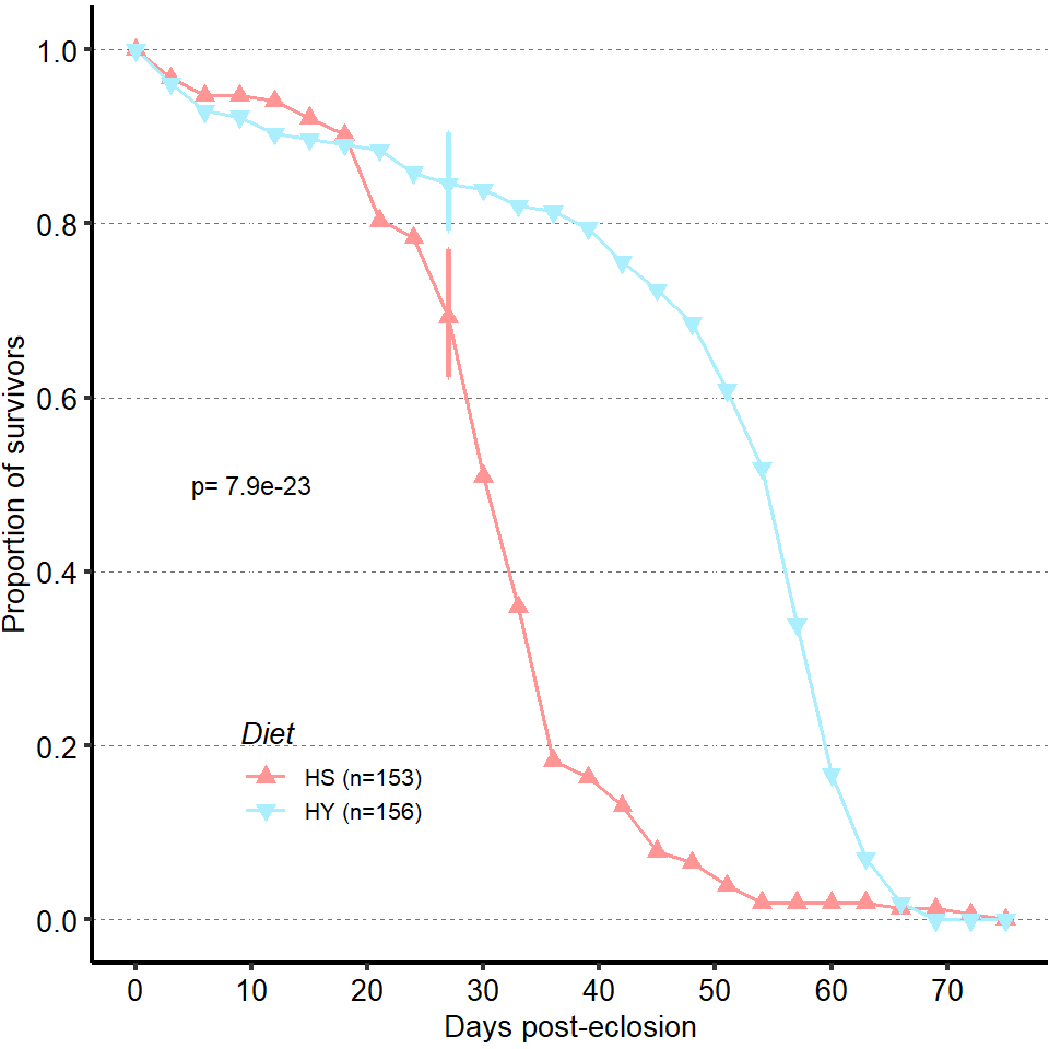
##Export Figure 5S1
5.3 Figure 5 - supplementary 2
5.3.1 Figure 5S2A-D’
p-eIF2α stain is elevated in all cells of the epithelium on HS (A, A’, first row) diet compared to HY (B,B’, second row) diet, and less strongly in visceral muscle (C-D’, third row HS, fourth row HY). In red anti p-eIF2α stain together with EsgTS>UAS-GFP in green (progenitor cells marker) in A, B, or alone in A’, B’. A to B’ are maximum intensity projection of z-stack. In red anti p-eIF2α stain together with HowTS>UAS-GFP in green (Visceral muscle marker) in C, D, or alone in C’, D’ (Single z-stack). Complete graphical annotation can be found in manuscript figures
img = readImage("F:/Dropbox/Github/Bonfini_eLife_2021/data/5 - S2A.jpg")
gob_imageFig5S2A = rasterGrob(img)
grid.draw(gob_imageFig5S2A)
img = readImage("F:/Dropbox/Github/Bonfini_eLife_2021/data/5 - S2A'.jpg")
gob_imageFig5S2A1 = rasterGrob(img)
grid.draw(gob_imageFig5S2A1)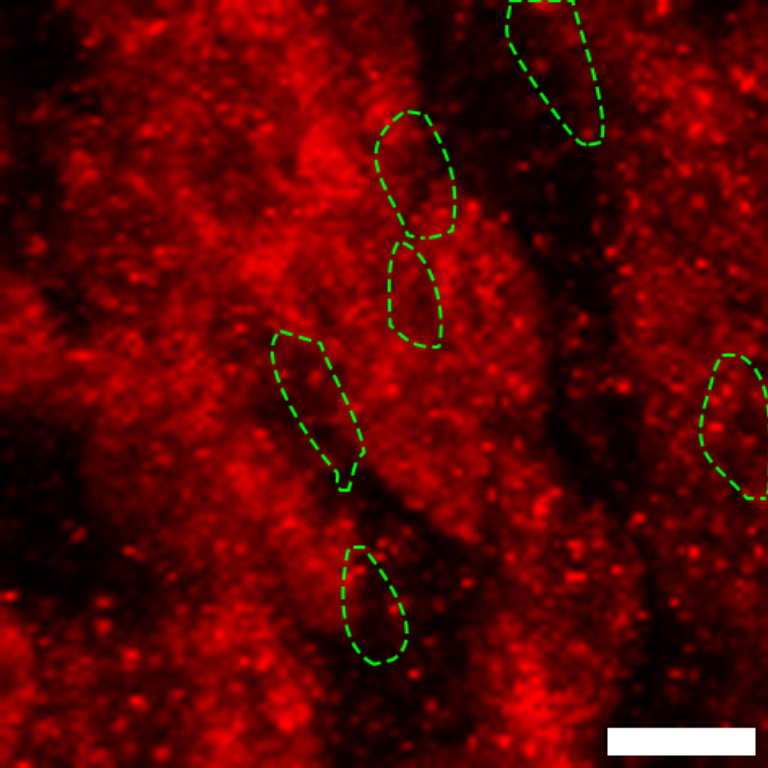
img = readImage("F:/Dropbox/Github/Bonfini_eLife_2021/data/5 - S2B.jpg")
gob_imageFig5S2B = rasterGrob(img)
grid.draw(gob_imageFig5S2B)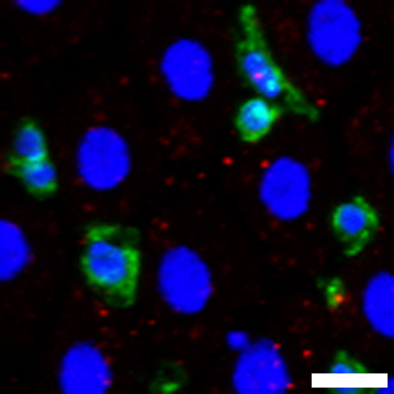
img = readImage("F:/Dropbox/Github/Bonfini_eLife_2021/data/5 - S2B'.jpg")
gob_imageFig5S2B1 = rasterGrob(img)
grid.draw(gob_imageFig5S2B1)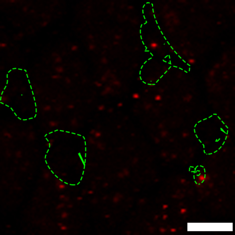
img = readImage("F:/Dropbox/Github/Bonfini_eLife_2021/data/5 - S2C.jpg")
gob_imageFig5S2C = rasterGrob(img)
grid.draw(gob_imageFig5S2C)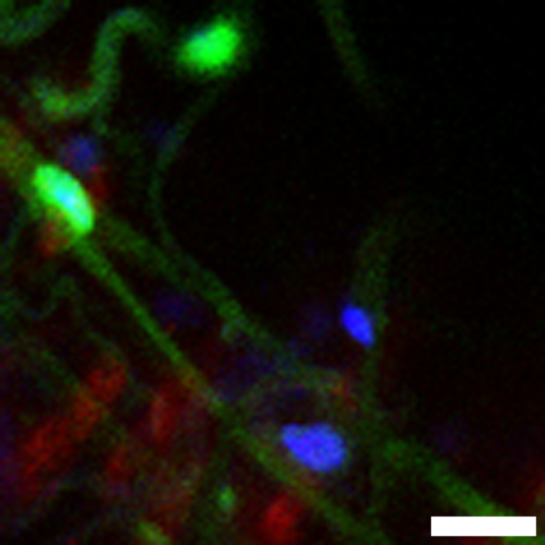
img = readImage("F:/Dropbox/Github/Bonfini_eLife_2021/data/5 - S2C'.jpg")
gob_imageFig5S2C1 = rasterGrob(img)
grid.draw(gob_imageFig5S2C1)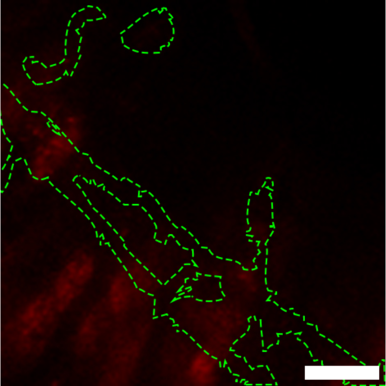
img = readImage("F:/Dropbox/Github/Bonfini_eLife_2021/data/5 - S2D.jpg")
gob_imageFig5S2D = rasterGrob(img)
grid.draw(gob_imageFig5S2D)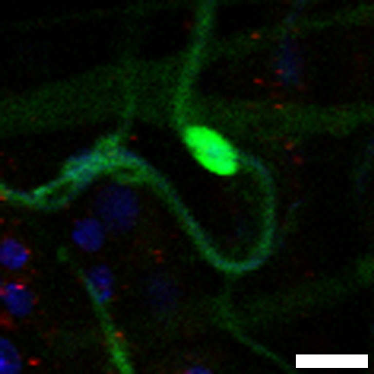
img = readImage("F:/Dropbox/Github/Bonfini_eLife_2021/data/5 - S2D'.jpg")
gob_imageFig5S2D1 = rasterGrob(img)
grid.draw(gob_imageFig5S2D1)
5.3.2 Figure 5S2E
Blocking translational inhibition with ActTS>Gcn2-IR or ActTS>LK6-IR is sufficient to increase pH3+ cells in midguts of flies shifted from HY to HS diet. However, ActTS>PEK-IR and ActTS>AMPKα-IR had no effect on the number of pH3+ cells. Statistical comparisons are vs control.
tab_PH3_Translation =
d[["5 - S2E"]]%>%
mutate_at(vars(!starts_with("Total")),as.factor)%>%
dplyr::rename(PH3_positive_cell=Total.PH3,
Day_of_treatment=Day)
Sample_size=
tab_PH3_Translation%>%
group_by(Male.Line)%>%
summarise(Sample_size=n())
###Stats
#Gcn2-IR
tmp = subset(tab_PH3_Translation,!is.na(PH3_positive_cell) & Male.Line%in%c("Control","Gcn2-IR"))
mod.gen = fitme(log(PH3_positive_cell+1) ~ Male.Line + (1 | Repeat),data = tmp)
shapiro.test(residuals(mod.gen))
Shapiro-Wilk normality test
data: residuals(mod.gen)
W = 0.95985, p-value = 0.1131bptest(log(PH3_positive_cell+1) ~ Male.Line + (1 / Repeat),data = tmp)
studentized Breusch-Pagan test
data: log(PH3_positive_cell + 1) ~ Male.Line + (1/Repeat)
BP = 3.0597, df = 1, p-value = 0.08026mod.gen1 = fitme(log(PH3_positive_cell+1) ~ 1 + (1 | Repeat),data = tmp)
test = anova(mod.gen, mod.gen1)
Chi2_LRT_growth = 2*(mod.gen$APHLs[["p_v"]]-mod.gen1$APHLs[["p_v"]])
tab_stat = data.frame(Male.Line = as.character(paste("Control vs Gcn2-IR")),
Rep = nlevels(tmp$Repeat),
chi2_LR = round(as.numeric(test$basicLRT$chi2_LR), digits = 2),
intercept = format(mod.gen$fixef[1],digits=3),
estimate = format(mod.gen$fixef[2],digits=3),
df = as.numeric(test$basicLRT$df),
Pvalue = as.numeric(format(pchisq(Chi2_LRT_growth,df=1,lower.tail = F),digits=2)))
tab_stat_GCN=tab_stat
#PEK-IR
tmp = subset(tab_PH3_Translation,!is.na(PH3_positive_cell) & Male.Line%in%c("Control","PEK-IR"))
mod.gen = fitme(log(PH3_positive_cell+1) ~ Male.Line + (1 | Repeat),data = tmp)
shapiro.test(residuals(mod.gen))
Shapiro-Wilk normality test
data: residuals(mod.gen)
W = 0.96541, p-value = 0.2422bptest(log(PH3_positive_cell+1) ~ Male.Line + (1 / Repeat),data = tmp)
studentized Breusch-Pagan test
data: log(PH3_positive_cell + 1) ~ Male.Line + (1/Repeat)
BP = 0.28498, df = 1, p-value = 0.5935mod.gen1 = fitme(log(PH3_positive_cell+1) ~ 1 + (1 | Repeat),data = tmp)
test = anova(mod.gen, mod.gen1)
Chi2_LRT_growth = 2*(mod.gen$APHLs[["p_v"]]-mod.gen1$APHLs[["p_v"]])
tab_stat = data.frame(Male.Line = as.character(paste("Control vs PEK-IR")),
Rep = nlevels(tmp$Repeat),
chi2_LR = round(as.numeric(test$basicLRT$chi2_LR), digits = 2),
intercept = format(mod.gen$fixef[1],digits=3),
estimate = format(mod.gen$fixef[2],digits=3),
df = as.numeric(test$basicLRT$df),
Pvalue = as.numeric(format(pchisq(Chi2_LRT_growth,df=1,lower.tail = F),digits=1,scientific=F)))
tab_stat_PEK=tab_stat
#Lk6-IR
tmp = subset(tab_PH3_Translation,!is.na(PH3_positive_cell) & Male.Line%in%c("Control","Lk6-IR"))
mod.gen = fitme(log(PH3_positive_cell+1) ~ Male.Line + (1 | Repeat),data = tmp)
shapiro.test(residuals(mod.gen))
Shapiro-Wilk normality test
data: residuals(mod.gen)
W = 0.98726, p-value = 0.8899bptest(log(PH3_positive_cell+1) ~ Male.Line + (1 / Repeat),data = tmp)
studentized Breusch-Pagan test
data: log(PH3_positive_cell + 1) ~ Male.Line + (1/Repeat)
BP = 1.2795, df = 1, p-value = 0.258mod.gen1 = fitme(log(PH3_positive_cell+1) ~ 1 + (1 | Repeat),data = tmp)
test = anova(mod.gen, mod.gen1)
Chi2_LRT_growth = 2*(mod.gen$APHLs[["p_v"]]-mod.gen1$APHLs[["p_v"]])
tab_stat = data.frame(Male.Line = as.character(paste("Control vs Lk6-IR")),
Rep = nlevels(tmp$Repeat),
chi2_LR = round(as.numeric(test$basicLRT$chi2_LR), digits = 2),
intercept = format(mod.gen$fixef[1],digits=3),
estimate = format(mod.gen$fixef[2],digits=3),
df = as.numeric(test$basicLRT$df),
Pvalue = as.numeric(format(pchisq(Chi2_LRT_growth,df=1,lower.tail = F),digits=2)))
tab_stat_Lk6=tab_stat
#Ampk-IR
tmp = subset(tab_PH3_Translation,!is.na(PH3_positive_cell) & Male.Line%in%c("Control","Ampk-IR"))
tmp$Male.Line = factor(tmp$Male.Line,levels = c("Control","Ampk-IR"))
mod.gen = fitme(log(PH3_positive_cell+1) ~ Male.Line + (1 | Repeat),data = tmp)
shapiro.test(residuals(mod.gen))
Shapiro-Wilk normality test
data: residuals(mod.gen)
W = 0.9837, p-value = 0.7479bptest(log(PH3_positive_cell+1) ~ Male.Line + (1 / Repeat),data = tmp)
studentized Breusch-Pagan test
data: log(PH3_positive_cell + 1) ~ Male.Line + (1/Repeat)
BP = 0.13265, df = 1, p-value = 0.7157mod.gen1 = fitme(log(PH3_positive_cell+1) ~ 1 + (1 | Repeat),data = tmp)
test = anova(mod.gen, mod.gen1)
Chi2_LRT_growth = 2*(mod.gen$APHLs[["p_v"]]-mod.gen1$APHLs[["p_v"]])
tab_stat = data.frame(Male.Line = as.character(paste("Control vs Ampk-IR")),
Rep = nlevels(tmp$Repeat),
chi2_LR = round(as.numeric(test$basicLRT$chi2_LR), digits = 2),
intercept = format(mod.gen$fixef[1],digits=3),
estimate = format(mod.gen$fixef[2],digits=3),
df = as.numeric(test$basicLRT$df),
Pvalue = as.numeric(format(pchisq(Chi2_LRT_growth,df=1,lower.tail = F),digits=1,scientific=F)))
tab_stat_Ampk=tab_stat
tab_stat=rbind(tab_stat_PEK,tab_stat_Ampk,tab_stat_Lk6,tab_stat_GCN)
letter_position = aggregate(data=tab_PH3_Translation,PH3_positive_cell ~ Male.Line, max)
tab_stat=left_join(tab_stat,letter_position)
tab_stat$padj = as.numeric(format(p.adjust(tab_stat$Pvalue, method = "BH"),digits=2,scientific =T))
tab_stat$sig = ifelse(tab_stat$padj < 0.05 & tab_stat$padj > 0.01, "*",
ifelse(tab_stat$padj < 0.01 & tab_stat$padj > 0.001, "**",
ifelse(tab_stat$padj < 0.001, "***", "")))
tab_stat%>%
kable(col.names = c("Comparison", "Replicates", "Chi2","Intercept","Estimate","df" ,"p-value","letter position","p-value adjusted","Signif."),row.names = FALSE) %>%
add_header_above(c("log(PH3_positive_cell+1) ~ Genotype + (1 | Repeat)" = 10))%>%
kable_styling(bootstrap_options = c("striped", "hover", "condensed"), full_width = F)| Comparison | Replicates | Chi2 | Intercept | Estimate | df | p-value | letter position | p-value adjusted | Signif. |
|---|---|---|---|---|---|---|---|---|---|
| Control vs PEK-IR | 3 | 0.63 | 2.08 | 0.188 | 1 | 4e-01 | NA | 5.3e-01 | |
| Control vs Ampk-IR | 3 | 0.02 | 2.07 | -0.0243 | 1 | 9e-01 | NA | 9.0e-01 | |
| Control vs Lk6-IR | 3 | 26.82 | 2.07 | 1.06 | 1 | 2e-07 | NA | 4.0e-07 | *** |
| Control vs Gcn2-IR | 3 | 29.80 | 2.09 | 1.17 | 1 | 0e+00 | NA | 2.0e-07 | *** |
tab_stat5S2E = tab_stat
### Plot
tab_PH3_Translation$Female.Line = factor(tab_PH3_Translation$Female.Line, labels = c(expression(italic(paste("Ac",t^{TS},">",sep="")))))
z=max(tab_PH3_Translation$PH3_positive_cell, na.rm = TRUE)
Plot_Fig5S2E=
ggplot(tab_PH3_Translation, aes(x = Male.Line, y = PH3_positive_cell))+
geom_violin(aes(fill = Diet), draw_quantiles = c(0.25, 0.5, 0.75), colour = "black", size = 0.2,adjust = 0.8) +
geom_dotplot( colour = "black", fill = "white", binaxis = "y", stackdir = "center", binwidth = z/40) +
geom_text(data = Sample_size, mapping = aes(x = Male.Line, y = -3, label = paste("(",Sample_size,")",sep="")),size=3)+
facet_grid(.~Female.Line, labeller = label_parsed)+
scale_fill_manual(values="#FFE5E5")+
scale_x_discrete("",
limits=c("Control", "Ampk-IR", "PEK-IR", "Gcn2-IR","Lk6-IR"),
labels=c(expression(italic("Control"), italic(paste("AMPK", alpha, "-IR")), italic("PEK-IR"), italic("Gcn2-IR"), italic("Lk6-IR"))))+
scale_y_continuous(expression(paste("pH3" ^ "+", " cells")),
limits=c(-3,64),
breaks=seq(0,62,by=20))+
stat_summary(fun = mean, geom = "point", size = 3, shape = 18, colour = "black", aes(group = Repeat)) +
stat_summary(fun = mean, geom = "point", size = 2, shape = 18, aes(group = Repeat, colour = Repeat)) +
scale_color_manual(values = palette_mean) +
theme(panel.grid.major.y = element_line(colour = grey(0.45), linetype = "dashed", size = 0.2),
panel.background = element_blank(),
axis.title.x = element_text(size=Smallfont,colour="black", face = "italic"),
axis.title.y = element_text(size=Smallfont,colour="black"),
axis.line.x = element_line(colour="black",size=0.75),
axis.line.y = element_line(colour="black",size=0.75),
axis.ticks.x = element_line(size = 0.75),
axis.ticks.y = element_line(size = 0.75),
axis.text.x = element_text(size=Smallfont,colour="black",angle=30,hjust=1),
axis.text.y = element_text(size=Smallfont,colour="black"),
plot.margin = unit(Margin, "cm"),
legend.direction = "vertical",
legend.box = "horizontal",
legend.position = "none",
legend.key.height = unit(0.4, "cm"),
legend.key.width= unit(0.6, "cm"),
legend.title = element_text(face="italic",size=Smallfont),
legend.key = element_rect(colour = 'white', fill = "white", linetype='dashed'),
legend.text = element_text(size=SuperSmallfont),
legend.background = element_rect(fill=NA),
strip.text.x = element_text(size = Smallfont, colour = "black", margin = margin(t = 2, r = 0, b = 2, l = 0)),
strip.text.y = element_text(size = Smallfont, colour = "black", margin = margin(t = 2, r = 0, b = 2, l = 0)),
strip.background = element_rect(fill=NA, colour="black"),
strip.placement="outside")
Plot_Fig5S2E
5.3.3 Figure 5S2F
Despite increased mitotic activity following repression of translational inhibition in ActTS>Gcn2-IR or ActTS>LK6-IR, midgut size was still shrinking on flies shifted from HY to HS diet for 7 days. The statistical comparison is comparing interaction between diet and fly lines. Complete statistical annotation on image can be found in the manuscript’s figure.
tab_length_Translation =
d[["5 - S2F"]]%>%
mutate_at(vars(!starts_with("Total")),as.factor)%>%
mutate(Total_Length_mm=Total.L/1000)%>%
dplyr::rename(Day_of_treatment=Day,
Female_Line=Female.Line,
Male_Line=Male.Line)%>%
as.data.frame()%>%
mutate(Male_Line=fct_relevel(Male_Line,c("Control","Gcn2-IR","Lk6-IR")))
Sample_size=
tab_length_Translation%>%
group_by(Diet,Male_Line)%>%
summarise(Sample_size=n())
###Stats
#Gcn2-IR
tmp = subset(tab_length_Translation, Male_Line%in%c("Control","Gcn2-IR"))
mod.gen = fitme(log(Total_Length_mm) ~ Diet * Male_Line + (1 | Repeat),data = tmp)
shapiro.test(residuals(mod.gen))
Shapiro-Wilk normality test
data: residuals(mod.gen)
W = 0.99166, p-value = 0.8546bptest(log(Total_Length_mm) ~ Diet + Male_Line + (1 / Repeat),data = tmp)
studentized Breusch-Pagan test
data: log(Total_Length_mm) ~ Diet + Male_Line + (1/Repeat)
BP = 4.3162, df = 2, p-value = 0.1155mod.gen1 = fitme(log(Total_Length_mm) ~ Diet + Male_Line + (1 | Repeat),data = tmp)
test = anova(mod.gen, mod.gen1)
Chi2_LRT_growth = 2*(mod.gen$APHLs[["p_v"]]-mod.gen1$APHLs[["p_v"]])
tab_stat = data.frame(Male_Line = as.character(paste("Control interaction vs Gcn2-IR interaction")),
Rep = nlevels(tmp$Repeat),
chi2_LR = round(as.numeric(test$basicLRT$chi2_LR), digits = 2),
intercept = format(mod.gen$fixef[1],digits=3),
estimate = format(mod.gen$fixef[2],digits=3),
df = as.numeric(test$basicLRT$df),
Pvalue = as.numeric(format(pchisq(Chi2_LRT_growth,df=1,lower.tail = F),digits=1,scientific=F)))
tab_stat_Gcn2=tab_stat
#Lk6-IR
tmp = subset(tab_length_Translation, Male_Line%in%c("Control","Lk6-IR"))
mod.gen = fitme(log(Total_Length_mm) ~ Diet * Male_Line + (1 | Repeat),data = tmp)
shapiro.test(residuals(mod.gen))
Shapiro-Wilk normality test
data: residuals(mod.gen)
W = 0.99083, p-value = 0.8181bptest(log(Total_Length_mm) ~ Diet + Male_Line + (1 / Repeat),data = tmp)
studentized Breusch-Pagan test
data: log(Total_Length_mm) ~ Diet + Male_Line + (1/Repeat)
BP = 0.69052, df = 2, p-value = 0.708mod.gen1 = fitme(log(Total_Length_mm) ~ Diet + Male_Line + (1 | Repeat),data = tmp)
test = anova(mod.gen, mod.gen1)
Chi2_LRT_growth = 2*(mod.gen$APHLs[["p_v"]]-mod.gen1$APHLs[["p_v"]])
tab_stat = data.frame(Male_Line = as.character(paste("Control interaction vs Lk6-IR interaction")),
Rep = nlevels(tmp$Repeat),
chi2_LR = round(as.numeric(test$basicLRT$chi2_LR), digits = 2),
intercept = format(mod.gen$fixef[1],digits=3),
estimate = format(mod.gen$fixef[2],digits=3),
df = as.numeric(test$basicLRT$df),
Pvalue = as.numeric(format(pchisq(Chi2_LRT_growth,df=1,lower.tail = F),digits=1,scientific=F)))
tab_stat_Lk6=tab_stat
tab_stat=rbind(tab_stat_Lk6,tab_stat_Gcn2)
tab_stat$padj = as.numeric(format(p.adjust(tab_stat$Pvalue, method = "BH"),digits=2,scientific =F))
tab_stat$sig = ifelse(tab_stat$padj < 0.05 & tab_stat$padj > 0.01, "*",
ifelse(tab_stat$padj < 0.01 & tab_stat$padj > 0.001, "**",
ifelse(tab_stat$padj < 0.001, "***", "")))
tab_stat%>%
kable(col.names = c("Copparison", "Replicates", "Chi2","Intercept","Estimate","df" ,"p-value","p-value adjusted","Signif."),row.names = FALSE) %>%
add_header_above(c("log(Total_Length_mm) ~ Diet + Genotype + Diet : Genotype + (1 | Repeat)" = 9))%>%
kable_styling(bootstrap_options = c("striped", "hover", "condensed"), full_width = F)| Copparison | Replicates | Chi2 | Intercept | Estimate | df | p-value | p-value adjusted | Signif. |
|---|---|---|---|---|---|---|---|---|
| Control interaction vs Lk6-IR interaction | 3 | 3.71 | 1.78 | -0.23 | 1 | 0.05 | 0.06 | |
| Control interaction vs Gcn2-IR interaction | 3 | 3.61 | 1.78 | -0.224 | 1 | 0.06 | 0.06 |
tab_stat5S2F = tab_stat
### Plot
tab_length_Translation$Female_Line = factor(tab_length_Translation$Female_Line, labels = c(expression(italic(paste("Ac",t^{TS},">",sep="")))))
Plot_Fig5S2F=
ggplot(tab_length_Translation, aes(x = Diet, y = Total_Length_mm))+
geom_violin(aes(fill = Diet), draw_quantiles = c(0.25, 0.5, 0.75), colour = "black", size = 0.2,adjust = 0.8) +
geom_dotplot( colour = "black", fill = "white", binaxis = "y", stackdir = "center", binwidth = 0.15) +
geom_text(data = Sample_size, mapping = aes(x = Diet, y = 2.5, label = paste("(",Sample_size,")",sep="")),size=3)+
facet_grid(.~ Male_Line)+
scale_fill_manual(values=c("#C3E6FC", "#FFE5E5"))+
scale_x_discrete("",
limits=c("HY D0","HYtoHS D7"),
labels=c("HY","HY to HS"))+
scale_y_continuous("Midgut length (mm)",
limits=c(2,9),
breaks=seq(2,8,by=1))+
stat_summary(fun = mean, geom = "point", size = 3, shape = 18, colour = "black", aes(group = Repeat)) +
stat_summary(fun = mean, geom = "point", size = 2, shape = 18, aes(group = Repeat, colour = Repeat)) +
stat_summary(fun = mean, colour = "black", geom = "line", aes(group = Repeat)) +
scale_color_manual(values = palette_mean) +
theme(panel.grid.major.y = element_line(colour = grey(0.45), linetype = "dashed", size = 0.2),
panel.background = element_blank(),
axis.title.x = element_text(size=Smallfont,colour="black"),
axis.title.y = element_text(size=Smallfont,colour="black"),
axis.line.x = element_line(colour="black",size=0.75),
axis.line.y = element_line(colour="black",size=0.75),
axis.ticks.x = element_line(size = 0.75),
axis.ticks.y = element_line(size = 0.75),
axis.text.x = element_text(size=Smallfont,colour="black",angle=30,hjust=1),
axis.text.y = element_text(size=Smallfont,colour="black"),
plot.margin = unit(Margin, "cm"),
legend.direction = "vertical",
legend.box = "horizontal",
legend.position = "none",
legend.key.height = unit(0.4, "cm"),
legend.key.width= unit(0.6, "cm"),
legend.title = element_text(face="italic",size=Smallfont),
legend.key = element_rect(colour = 'white', fill = "white", linetype='dashed'),
legend.text = element_text(size=SuperSmallfont),
legend.background = element_rect(fill=NA),
strip.text.x = element_text(size = Smallfont, colour = "black", margin = margin(t = 2, r = 0, b = 2, l = 0),face = "italic"),
strip.text.y = element_text(size = Smallfont, colour = "black", margin = margin(t = 2, r = 0, b = 2, l = 0), face = "italic"),
strip.background = element_rect(fill=NA, colour="black"),
strip.placement="outside")
Plot_Fig5S2F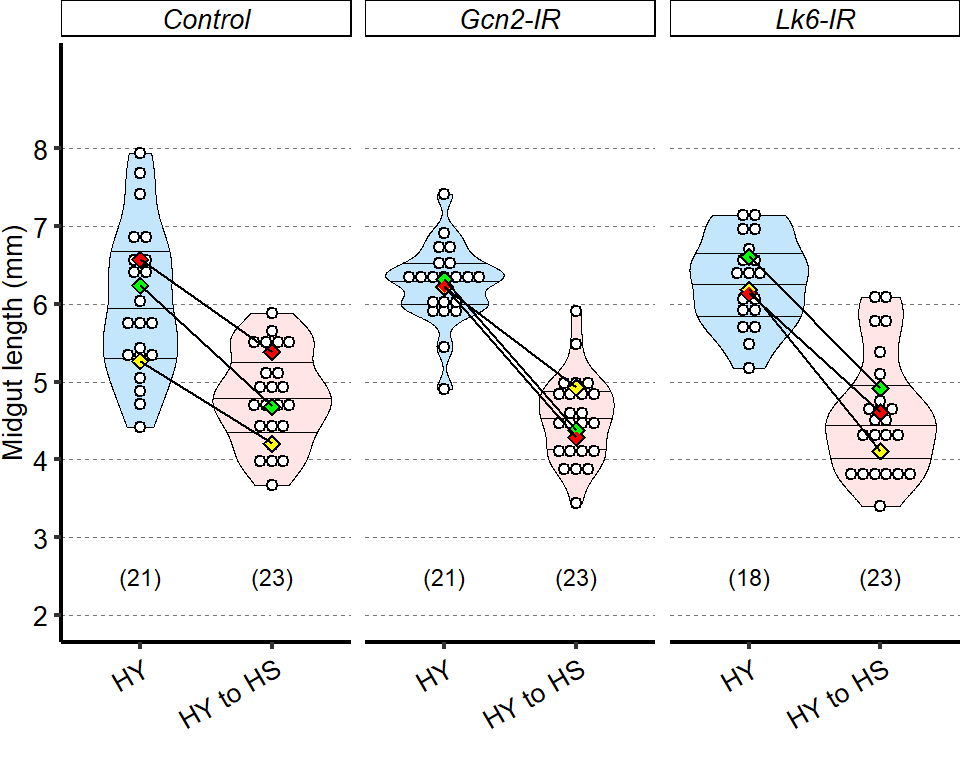
5.3.4 Figure 5S2G
Knockdown of Gcn2 in ECs (MyoTS>Gcn2-IR), but not in progenitor cells (EsgTS>Gcn2-IR), is sufficient to increase pH3+ cells in midguts of flies shifted after 12 days from eclosion on HY to HS diet for additional 7 days. Statistical comparisons are vs respective controls.
tab_PH3_Translation1 =
d[["5 - S2G"]]%>%
mutate_at(vars(!starts_with("Total")),as.factor)%>%
dplyr::rename(PH3_positive_cell=Total.PH3,
Day_of_treatment=Day)
Sample_size=
tab_PH3_Translation1%>%
group_by(Female.Line, Male.Line)%>%
summarise(Sample_size=n())
###Stats
#Esg
tmp = subset(tab_PH3_Translation1,!is.na(PH3_positive_cell) & Female.Line%in%c("Esg"))
mod.gen = fitme(log(PH3_positive_cell+1) ~ Male.Line + (1 | Repeat),data = tmp)
shapiro.test(residuals(mod.gen))
Shapiro-Wilk normality test
data: residuals(mod.gen)
W = 0.96868, p-value = 0.1948bptest(log(PH3_positive_cell+1) ~ Male.Line + (1 / Repeat),data = tmp)
studentized Breusch-Pagan test
data: log(PH3_positive_cell + 1) ~ Male.Line + (1/Repeat)
BP = 0.76503, df = 1, p-value = 0.3818mod.gen1 = fitme(log(PH3_positive_cell+1) ~ 1 + (1 | Repeat),data = tmp)
test = anova(mod.gen, mod.gen1)
Chi2_LRT_growth = 2*(mod.gen$APHLs[["p_v"]]-mod.gen1$APHLs[["p_v"]])
tab_stat = data.frame(Comparison = as.character(paste("Control vs Gcn2-IR EsgTS")),
Male.Line = as.character(paste("EsgTS x Gcn2-IR")),
Rep = nlevels(tmp$Repeat),
chi2_LR = round(as.numeric(test$basicLRT$chi2_LR), digits = 2),
intercept = format(mod.gen$fixef[1],digits=3),
estimate = format(mod.gen$fixef[2],digits=3),
df = as.numeric(test$basicLRT$df),
Pvalue = as.numeric(format(pchisq(Chi2_LRT_growth,df=1,lower.tail = F),digits=2)),
Female.Line = "Esg",
Male.line ="Gcn2-IR")
tab_stat_esg=tab_stat
#Myo
tmp = subset(tab_PH3_Translation1,!is.na(PH3_positive_cell) & Female.Line%in%c("Myo"))
mod.gen = fitme(log(PH3_positive_cell+1) ~ Male.Line + (1 | Repeat),data = tmp)
shapiro.test(residuals(mod.gen))
Shapiro-Wilk normality test
data: residuals(mod.gen)
W = 0.96482, p-value = 0.1495bptest(log(PH3_positive_cell+1) ~ Male.Line + (1 / Repeat),data = tmp)
studentized Breusch-Pagan test
data: log(PH3_positive_cell + 1) ~ Male.Line + (1/Repeat)
BP = 1.4773, df = 1, p-value = 0.2242mod.gen1 = fitme(log(PH3_positive_cell+1) ~ 1 + (1 | Repeat),data = tmp)
test = anova(mod.gen, mod.gen1)
Chi2_LRT_growth = 2*(mod.gen$APHLs[["p_v"]]-mod.gen1$APHLs[["p_v"]])
tab_stat = data.frame(Comparison = as.character(paste("Control vs Gcn2-IR EsgTS")),
Male.Line = as.character(paste("MyoTS x Gcn2-IR")),
Rep = nlevels(tmp$Repeat),
chi2_LR = round(as.numeric(test$basicLRT$chi2_LR), digits = 2),
intercept = format(mod.gen$fixef[1],digits=3),
estimate = format(mod.gen$fixef[2],digits=3),
df = as.numeric(test$basicLRT$df),
Pvalue = as.numeric(format(pchisq(Chi2_LRT_growth,df=1,lower.tail = F),digits=2)),
Female.Line = "Myo",
Male.line ="Gcn2-IR")
tab_stat_myo=tab_stat
#Table making
tab_stat=rbind(tab_stat_esg,tab_stat_myo)
tab_stat$sig = ifelse(tab_stat$Pvalue < 0.05 & tab_stat$Pvalue > 0.01, "*",
ifelse(tab_stat$Pvalue < 0.01 & tab_stat$Pvalue > 0.001, "**",
ifelse(tab_stat$Pvalue < 0.001, "***", "")))
tab_stat%>%
kable(col.names = c("Comparison", "Variable", "Replicates", "Chi2","Intercept","Estimate","df" ,"p-value","Female.Line","Male.Line","Signif."),row.names = FALSE) %>%
add_header_above(c("log(PH3_positive_cell+1) ~ Genotype + (1 | Repeat)" = 11))%>%
kable_styling(bootstrap_options = c("striped", "hover", "condensed"), full_width = F)| Comparison | Variable | Replicates | Chi2 | Intercept | Estimate | df | p-value | Female.Line | Male.Line | Signif. |
|---|---|---|---|---|---|---|---|---|---|---|
| Control vs Gcn2-IR EsgTS | EsgTS x Gcn2-IR | 3 | 2.45 | 2.04 | 0.354 | 1 | 1.2e-01 | Esg | Gcn2-IR | |
| Control vs Gcn2-IR EsgTS | MyoTS x Gcn2-IR | 3 | 20.73 | 2.59 | 0.828 | 1 | 5.3e-06 | Myo | Gcn2-IR | *** |
tab_stat5S2G = tab_stat
### Plot
tab_PH3_Translation1$Female.Line = factor(tab_PH3_Translation1$Female.Line, labels = c(expression(italic(paste("Es",g^{TS},">",sep=""))), expression(italic(paste("My",o^{TS},">",sep="")))))
tab_stat$Female.Line = tab_stat$Female.Line = factor(tab_stat$Female.Line, labels = c(expression(italic(paste("Es",g^{TS},">",sep=""))), expression(italic(paste("My",o^{TS},">",sep="")))))
Sample_size$Female.Line = Sample_size$Female.Line = factor(Sample_size$Female.Line, labels = c(expression(italic(paste("Es",g^{TS},">",sep=""))), expression(italic(paste("My",o^{TS},">",sep="")))))
z=max(tab_PH3_Translation1$PH3_positive_cell, na.rm = TRUE)
Plot_Fig5S2G=
ggplot(tab_PH3_Translation1, aes(x = Male.Line, y = PH3_positive_cell))+
geom_violin(aes(fill = Diet), draw_quantiles = c(0.25, 0.5, 0.75), colour = "black", size = 0.2,adjust = 0.8) +
geom_dotplot( colour = "black", fill = "white", binaxis = "y", stackdir = "center", binwidth = z/40) +
geom_text(data = Sample_size, mapping = aes(x = Male.Line, y = -4, label = paste("(",Sample_size,")",sep="")),size=3)+
facet_grid(.~Female.Line, labeller = label_parsed)+
scale_fill_manual(values="#FFE5E5")+
scale_x_discrete("",
limits=c("Control","Gcn2-IR"),
labels=c(expression(italic("Control"),italic("Gcn2-IR"))))+
scale_y_continuous(expression(paste("pH3" ^ "+", " cells")),
limits=c(-5,90),
breaks=seq(0,80,by=20))+
stat_summary(fun = mean, geom = "point", size = 3, shape = 18, colour = "black", aes(group = Repeat)) +
stat_summary(fun = mean, geom = "point", size = 2, shape = 18, aes(group = Repeat, colour = Repeat)) +
scale_color_manual(values = palette_mean) +
theme(panel.grid.major.y = element_line(colour = grey(0.45), linetype = "dashed", size = 0.2),
panel.background = element_blank(),
axis.title.x = element_text(size=Smallfont,colour="black", face = "italic"),
axis.title.y = element_text(size=Smallfont,colour="black"),
axis.line.x = element_line(colour="black",size=0.75),
axis.line.y = element_line(colour="black",size=0.75),
axis.ticks.x = element_line(size = 0.75),
axis.ticks.y = element_line(size = 0.75),
axis.text.x = element_text(size=Smallfont,colour="black",angle=30,hjust=1),
axis.text.y = element_text(size=Smallfont,colour="black"),
plot.margin = unit(Margin, "cm"),
legend.direction = "vertical",
legend.box = "horizontal",
legend.position = "none",
legend.key.height = unit(0.4, "cm"),
legend.key.width= unit(0.6, "cm"),
legend.title = element_text(face="italic",size=Smallfont),
legend.key = element_rect(colour = 'white', fill = "white", linetype='dashed'),
legend.text = element_text(size=SuperSmallfont),
legend.background = element_rect(fill=NA),
strip.text.x = element_text(size = Smallfont, colour = "black", margin = margin(t = 2, r = 0, b = 2, l = 0)),
strip.text.y = element_text(size = Smallfont, colour = "black", margin = margin(t = 2, r = 0, b = 2, l = 0)),
strip.background = element_rect(fill=NA, colour="black"),
strip.placement="outside")
Plot_Fig5S2G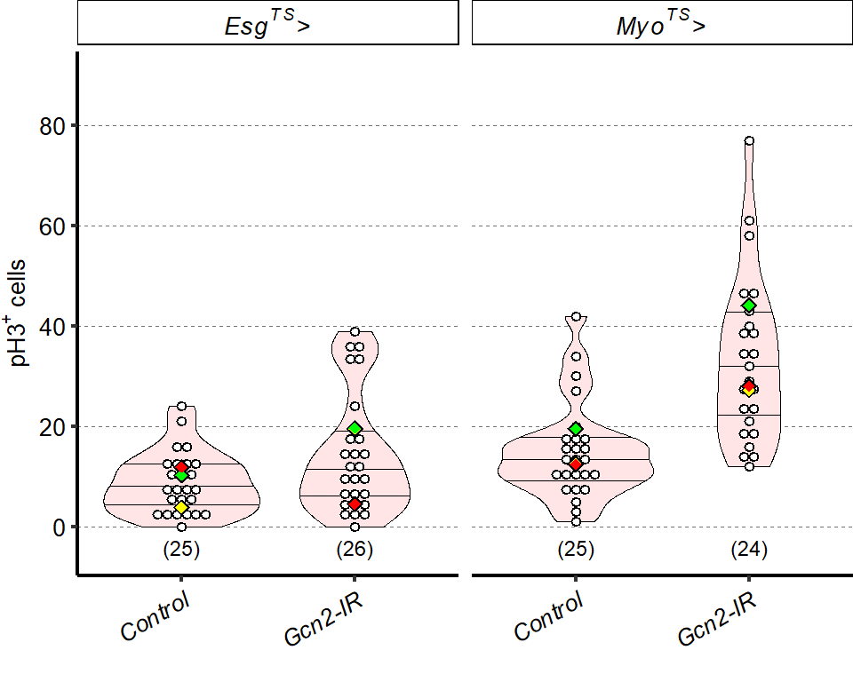
##Export Figure 5S2
6 Figure 6. The midgut can resize independently of stem cell proliferation
6.1 Figure 6 - main
6.1.1 Figure 6A
Mitotic index does not correlate with midgut length. Quantification of pH3+ cells across a selected panel of high and low responder DGRP lines shows that midgut length does not correlate with cell proliferation.
wolb = d[["DGRP_wolbachia_DFD"]]
colnames(wolb) = c("dgrp.id", "wolbachia")
wolb$dgrp.id = gsub("line_", "", wolb$dgrp.id)
tab_corr_length_cell_DGRP = subset(d[["6A - 7A"]])
tab_corr_length_cell_DGRP = merge(tab_corr_length_cell_DGRP, wolb, by.x="DGRP.number", by.y="dgrp.id", all.x=T, all.y=F)
colnames(tab_corr_length_cell_DGRP) = tolower(colnames(tab_corr_length_cell_DGRP))
colnames(tab_corr_length_cell_DGRP)[3] = "repl"
tab_corr_length_cell_DGRP$dgrp.number <- as.factor(tab_corr_length_cell_DGRP$dgrp.number)
tab_corr_length_cell_DGRP=
tab_corr_length_cell_DGRP%>%
dplyr::rename(ral=dgrp.number,
len=total.l,
ph3=total.ph3,
ec.area=area)%>%
mutate(ral=paste("Ral",ral,sep="_"))%>%
mutate_if(is.character,as.factor)
gut_mean=
tab_corr_length_cell_DGRP %>%
group_by(ral, diet,cross,gutnumber)%>%
summarize(mean_gut_len=mean(len,na.rm=T),
mean_cell_size=mean(ec.area,na.rm=T),
se_cell_size=sd(ec.area)/ sqrt(length(ec.area[!is.na(ec.area)])),
mean_PH3=mean(ph3,na.rm=T)) %>%
mutate(Group=paste(cross,gutnumber,sep="_"))
levels(gut_mean$ral) <- c("Ral 356", "Ral 362", "Ral 370", "Ral 502", "Ral 765", "Ral 853", "Ral 911")
gut_mean$ral <- factor(gut_mean$ral, levels = c("Ral 356", "Ral 502", "Ral 765", "Ral 853", "Ral 911", "Ral 362", "Ral 370"))
# stat over all
mod.gen = fitme(log10(I(mean_gut_len/1000)) ~ mean_PH3 + (1 | ral),data = gut_mean)
shapiro.test(residuals(mod.gen))
Shapiro-Wilk normality test
data: residuals(mod.gen)
W = 0.98787, p-value = 0.02606bptest(log10(I(mean_gut_len/1000)) ~ mean_PH3 + (1 / ral),data = gut_mean)
studentized Breusch-Pagan test
data: log10(I(mean_gut_len/1000)) ~ mean_PH3 + (1/ral)
BP = 0.085137, df = 1, p-value = 0.7705mod.gen1 = fitme(log10(I(mean_gut_len/1000)) ~ 1 + (1 | ral),data =gut_mean)
test = anova(mod.gen, mod.gen1)
Chi2_LRT_growth = 2*(mod.gen$APHLs[["p_v"]]-mod.gen1$APHLs[["p_v"]])
tab_stat = data.frame(Variable = as.character(paste("PH3 cell")),
Number_genotypes = nlevels(gut_mean$ral),
chi2_LR = round(as.numeric(test$basicLRT$chi2_LR), digits = 2),
intercept = format(mod.gen$fixef[1],digits=3),
estimate = format(mod.gen$fixef[2],digits=3),
df = as.numeric(test$basicLRT$df),
Pvalue = as.numeric(format(pchisq(Chi2_LRT_growth,df=1,lower.tail = F),digits=2)))
tab_stat$sig = ifelse(tab_stat$Pvalue < 0.05 & tab_stat$Pvalue > 0.01, "*",
ifelse(tab_stat$Pvalue < 0.01 & tab_stat$Pvalue > 0.001, "**",
ifelse(tab_stat$Pvalue < 0.001, "***", "")))
tab_stat%>%
kable(col.names = c("Variable", "Replicates", "Chi2","Intercept","Estimate","df" ,"p-value","Signif."),row.names = FALSE) %>% add_header_above(c("log10(I(mean_gut_len/1000)) ~ mean_PH3 + (1 | Genotype)" = 8))%>%
kable_styling(bootstrap_options = c("striped", "hover", "condensed"), full_width = F)| Variable | Replicates | Chi2 | Intercept | Estimate | df | p-value | Signif. |
|---|---|---|---|---|---|---|---|
| PH3 cell | 7 | 12.04 | 0.715 | -0.00121 | 1 | 0.00052 | *** |
#stat per line
Cor_PH3=NULL
for(i in unique(gut_mean$ral)){
#print(i)
cor_PH3_HS=
with(subset(gut_mean,ral==i& diet=="HS"),
cor.test(log(mean_gut_len,10),mean_PH3))
cor_PH3_HY=
with(subset(gut_mean,ral==i& diet=="HY"),
cor.test(log(mean_gut_len,10),mean_PH3))
Cor_PH3_tmp = data.frame(ral = as.character(i),
diet=c("HS","HY"),
Cor = c(format(as.numeric(cor_PH3_HS$estimate), digits = 2),format(as.numeric(cor_PH3_HY$estimate), digits = 2)),
Pvalue = c(format(as.numeric(cor_PH3_HS$p.value), digits = 2),format(as.numeric(cor_PH3_HY$p.value), digits = 2)))
Cor_PH3= rbind(Cor_PH3,Cor_PH3_tmp)
}
Cor_PH3$padj=p.adjust(Cor_PH3$Pvalue,method = "BH")
Cor_PH3$sig= ifelse(Cor_PH3$padj < 0.05 & Cor_PH3$padj > 0.01, "*",
ifelse(Cor_PH3$padj < 0.01 & Cor_PH3$padj > 0.001, "**",
ifelse(Cor_PH3$padj < 0.001, "***", "ns")))
tmp=subset(gut_mean,diet=="HS")
stat_position_HS = aggregate(data=tmp,mean_gut_len/1000 ~ ral, max)
stat_position_HS$diet="HS"
tmp=subset(gut_mean,diet=="HY")
stat_position_HY = aggregate(data=tmp,mean_gut_len/1000 ~ ral, max)
stat_position_HY$diet="HY"
stat_position=rbind(stat_position_HS,stat_position_HY)
colnames(stat_position)[2]="Stat_position"
Cor_PH3 = left_join(Cor_PH3,stat_position)
gut_mean$ral <- factor(gut_mean$ral, levels = c("Ral 356", "Ral 502", "Ral 765", "Ral 853", "Ral 911", "Ral 362", "Ral 370"))
Cor_PH3$ral <- factor(Cor_PH3$ral, levels = c("Ral 356", "Ral 502", "Ral 765", "Ral 853", "Ral 911", "Ral 362", "Ral 370"))
Sample_size=
gut_mean%>%
group_by(diet, ral)%>%
summarise(Sample_size=n())%>%
as.data.frame()%>%
mutate(ral=fct_relevel(ral,"Ral 356", "Ral 502", "Ral 765", "Ral 853", "Ral 911", "Ral 362", "Ral 370"))
cor_gut_PH3=
ggplot(gut_mean,aes(x=mean_PH3, y=mean_gut_len/1000,group=ral))+
geom_point(aes(color=diet,fill=diet),shape=21,size=0.9)+
geom_text(data = Sample_size, mapping = aes(x = 35, y = 2.5, label = paste("(",Sample_size,")",sep="")),size=3)+
geom_text(data = Cor_PH3, mapping = aes( x=60,y=7,label = sig),size=3)+
facet_grid(ral~diet)+
scale_y_continuous("Midgut length (mm)")+
scale_x_continuous(expression(paste("pH3" ^ "+", " cells")))+
scale_color_manual("",
limits=c("HS","HY"),
values=palette_diet_2)+
scale_fill_manual("",
limits=c("HS","HY"),
values=palette_diet_2)+
geom_smooth(method="lm",color="black",size=0.5)+
theme(panel.grid.major.y = element_line(colour = grey(0.45), linetype = "dashed", size = 0.2),
axis.title.x = element_text(size=Mediumfont,colour="black"),
axis.title.y = element_text(size=Mediumfont),
axis.line.x = element_line(colour="black"),
axis.line.y = element_line(colour="black"),
axis.ticks.x = element_line(),
axis.ticks.y = element_line(),
axis.text.x = element_text(size=Smallfont,colour="black"),
axis.text.y = element_text(size=Smallfont,colour="black"),
panel.grid = element_blank(),
plot.margin = unit(c(0,0,0,0), "cm"),
legend.direction = "vertical",
legend.box = "vertical",
legend.position = "none",
legend.key.height = unit(0.3, "cm"),
legend.key.width= unit(0.3, "cm"),
strip.text.x = element_text(size =Smallfont, colour = "black", margin = margin(t = 2, r = 0, b = 2, l = 0)),
strip.text.y = element_text(size =Smallfont, colour = "black",face="italic", margin = margin(t = 2, r = 0, b = 2, l = 0)),
strip.background = element_rect(color="black",fill=NA),
strip.placement="outside",
legend.title = element_text(face="italic",size=Smallfont),
legend.key = element_rect(colour = 'white', fill = "white", linetype='dashed'),
legend.text = element_text(size=Smallfont),
legend.background = element_rect(fill=NA),
panel.background = element_rect(fill="transparent"))+
guides(shape=guide_legend(ncol=1),
fill=guide_legend(ncol=1),
col=guide_legend(ncol=1))
cor_gut_PH3
6.1.2 Figure 6B-C
Blocking EGF signaling with UAS-Egfr-IR in progenitor cells (B, right) results in progenitor cells being almost wiped out compared to control (C, left).Complete graphical annotation can be found in manuscript figures
img = readImage("F:/Dropbox/Github/Bonfini_eLife_2021/data/6B.jpg")
gob_imageFig6B = rasterGrob(img)
grid.draw(gob_imageFig6B)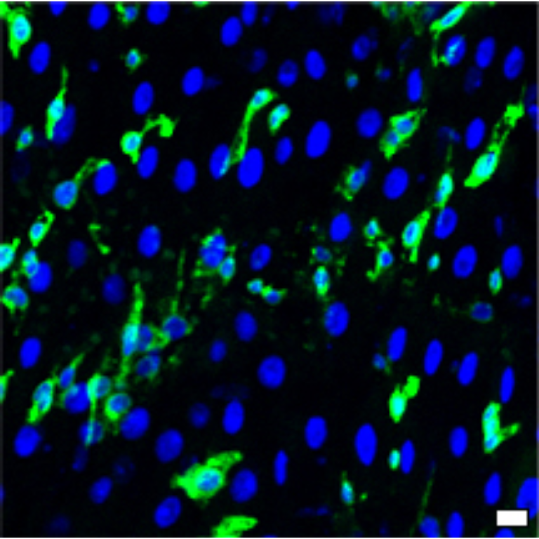
img = readImage("F:/Dropbox/Github/Bonfini_eLife_2021/data/6C.jpg")
gob_imageFig6C = rasterGrob(img)
grid.draw(gob_imageFig6C)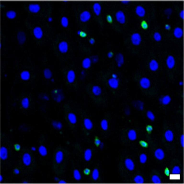
6.1.3 Figure 6D
pH3+ counts for EsgTS>Control vs EsgTS> EGFR-IR
tab_PH3_esg =
d[["6D"]]%>%
mutate_at(vars(!starts_with("Total")),as.factor)%>%
dplyr::rename(PH3_positive_cell=Total.PH3,
Day_of_treatment=Day)
Sample_size=
tab_PH3_esg%>%
group_by(Male.Line)%>%
summarise(Sample_size=n())
###Stats
mod.gen = fitme(PH3_positive_cell ~ Male.Line + (1 | Repeat),data = subset(tab_PH3_esg,!is.na(PH3_positive_cell)))
shapiro.test(residuals(mod.gen))
Shapiro-Wilk normality test
data: residuals(mod.gen)
W = 0.90554, p-value = 0.006445bptest(PH3_positive_cell ~ Male.Line + (1 / Repeat),data = subset(tab_PH3_esg,!is.na(PH3_positive_cell)))
studentized Breusch-Pagan test
data: PH3_positive_cell ~ Male.Line + (1/Repeat)
BP = 8.6215, df = 1, p-value = 0.003322mod.gen1 = fitme(PH3_positive_cell ~ 1 + (1 | Repeat),data = subset(tab_PH3_esg,!is.na(PH3_positive_cell)))
test = anova(mod.gen, mod.gen1)
Chi2_LRT_growth = 2*(mod.gen$APHLs[["p_v"]]-mod.gen1$APHLs[["p_v"]])
tab_stat = data.frame(Variable = as.character(paste("Control vs Egfr-IR")),
Rep = nlevels(tab_PH3_esg$Repeat),
chi2_LR = round(as.numeric(test$basicLRT$chi2_LR), digits = 2),
intercept = format(mod.gen$fixef[1],digits=3),
estimate = format(mod.gen$fixef[2],digits=3),
df = as.numeric(test$basicLRT$df),
Pvalue = as.numeric(format(pchisq(Chi2_LRT_growth,df=1,lower.tail = F),digits=2)))
tab_stat$sig = ifelse(tab_stat$Pvalue < 0.05 & tab_stat$Pvalue > 0.01, "*",
ifelse(tab_stat$Pvalue < 0.01 & tab_stat$Pvalue > 0.001, "**",
ifelse(tab_stat$Pvalue < 0.001, "***", "")))
tab_stat%>%
kable(col.names = c("Comparison", "Replicates", "Chi2","Intercept","Estimate","df" ,"p-value","Signif."),row.names = FALSE) %>% add_header_above(c("PH3_positive_cell ~ Genotype + (1 | Repeat)" = 8))%>%
kable_styling(bootstrap_options = c("striped", "hover", "condensed"), full_width = F)| Comparison | Replicates | Chi2 | Intercept | Estimate | df | p-value | Signif. |
|---|---|---|---|---|---|---|---|
| Control vs Egfr-IR | 2 | 20.45 | 7.21 | -6.63 | 1 | 6.1e-06 | *** |
### Plot
tab_PH3_esg$Female.Line = factor(tab_PH3_esg$Female.Line, labels = c(expression(italic(paste("Es",g^{TS},">",sep="")))))
Plot_Fig6D=
ggplot(tab_PH3_esg, aes(x = Male.Line, y = PH3_positive_cell))+
geom_boxplot(aes(fill = Diet), colour = "black", size = 0.2,outlier.shape = NA) +
geom_dotplot( colour = "black", fill = "white", binaxis = "y", stackdir = "center", binwidth = 0.2) +
geom_text(data = Sample_size, mapping = aes(x = Male.Line, y = -0.8, label = paste("(",Sample_size,")",sep="")),size=3)+
geom_signif(data = tab_stat,aes(xmin = 1, xmax = 2, annotations = formatC(paste("p=",Pvalue), digits = 2), y_position = 8.5), textsize = 3, vjust = -0.2, manual = TRUE, tip_length = c(0.01, 0.01))+
facet_grid(.~Female.Line, labeller = label_parsed)+
scale_fill_manual(values="#E5E5FF")+
scale_x_discrete("",
limits=c("Cs","Egfr-IR"),
labels=c("Control","Egfr-IR"))+
scale_y_continuous(expression(paste("pH3" ^ "+", " cells")),
limits=c(-1,9),
breaks=seq(0,8,by=2))+
stat_summary(fun = mean, geom = "point", size = 3, shape = 18, colour = "black", aes(group = Repeat)) +
stat_summary(fun = mean, geom = "point", size = 2, shape = 18, aes(group = Repeat, colour = Repeat)) +
scale_color_manual(values = palette_mean) +
theme(panel.grid.major.y = element_line(colour = grey(0.45), linetype = "dashed", size = 0.2),
panel.background = element_blank(),
axis.title.x = element_text(size=Smallfont,colour="black"),
axis.title.y = element_text(size=Smallfont,colour="black"),
axis.line.x = element_line(colour="black",size=0.75),
axis.line.y = element_line(colour="black",size=0.75),
axis.ticks.x = element_line(size = 0.75),
axis.ticks.y = element_line(size = 0.75),
axis.text.x = element_text(size=Smallfont,colour="black",angle=30,hjust=1, face = "italic"),
axis.text.y = element_text(size=Smallfont,colour="black"),
plot.margin = unit(Margin, "cm"),
legend.direction = "vertical",
legend.box = "horizontal",
legend.position = "none",
legend.key.height = unit(0.4, "cm"),
legend.key.width= unit(0.6, "cm"),
legend.title = element_text(face="italic",size=Smallfont),
legend.key = element_rect(colour = 'white', fill = "white", linetype='dashed'),
legend.text = element_text(size=SuperSmallfont),
legend.background = element_rect(fill=NA),
strip.text.x = element_text(size = Smallfont, colour = "black", face = "italic", margin = margin(t = 1, r = 0, b = 1, l = 0)),
strip.text.y = element_text(size = Smallfont, colour = "black", face = "italic", margin = margin(t = 1, r = 0, b = 1, l = 0)),
strip.background = element_rect(fill=NA, colour="black"),
strip.placement="outside")
Plot_Fig6D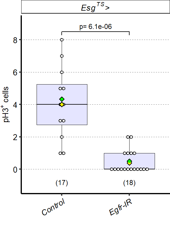
6.1.4 Figure 6E
EsgTS>UAS-Egfr-IR midguts are still able to reach a similar length to controls.
tab_length_esg =
d[["6E"]]%>%
mutate_at(vars(!starts_with("Total")),as.factor)%>%
mutate(Total_Length_mm=Total.L/1000)%>%
dplyr::rename(Day_of_treatment=Day,
Female_Line=Female.Line,
Male_Line=Male.Line)
Sample_size=
tab_length_esg%>%
group_by(Diet,Male_Line)%>%
summarise(Sample_size=n())
###Stats
mod.gen = fitme(log(Total_Length_mm) ~ Diet * Male_Line + (1 | Repeat),data = tab_length_esg)
shapiro.test(residuals(mod.gen))
Shapiro-Wilk normality test
data: residuals(mod.gen)
W = 0.98514, p-value = 0.2025bptest(log(Total_Length_mm) ~ Diet + Male_Line + (1 / Repeat),data = tab_length_esg)
studentized Breusch-Pagan test
data: log(Total_Length_mm) ~ Diet + Male_Line + (1/Repeat)
BP = 8.7188, df = 2, p-value = 0.01279mod.gen1 = fitme(log(Total_Length_mm) ~ Diet + Male_Line + (1 | Repeat),data = tab_length_esg)
test = anova(mod.gen, mod.gen1)
Chi2_LRT_growth = 2*(mod.gen$APHLs[["p_v"]]-mod.gen1$APHLs[["p_v"]])
tab_stat = data.frame(Variable = as.character(paste("Control vs Egfr-IR")),
Rep = nlevels(tab_length_esg$Repeat),
chi2_LR = round(as.numeric(test$basicLRT$chi2_LR), digits = 2),
intercept = format(mod.gen$fixef[1],digits=3),
estimate = format(mod.gen$fixef[2],digits=3),
df = as.numeric(test$basicLRT$df),
Pvalue = as.numeric(format(pchisq(Chi2_LRT_growth,df=1,lower.tail = F),digits=2)))
tab_stat$sig = ifelse(tab_stat$Pvalue < 0.05 & tab_stat$Pvalue > 0.01, "*",
ifelse(tab_stat$Pvalue < 0.01 & tab_stat$Pvalue > 0.001, "**",
ifelse(tab_stat$Pvalue < 0.001, "***", "")))
tab_stat%>%
kable(col.names = c("Comparison", "Replicates", "Chi2","Intercept","Estimate","df" ,"p-value","Signif."),row.names = FALSE) %>% add_header_above(c("log(Total_Length_mm) ~ Diet + Genotype + Diet : Genotype + (1 | Repeat)" = 8))%>%
kable_styling(bootstrap_options = c("striped", "hover", "condensed"), full_width = F)| Comparison | Replicates | Chi2 | Intercept | Estimate | df | p-value | Signif. |
|---|---|---|---|---|---|---|---|
| Control vs Egfr-IR | 4 | 0.27 | 1.51 | 0.375 | 1 | 0.6 |
tab_stat_6E=tab_stat
tab_stat_6E$Male_Line="Egfr-IR"
### Plot
tab_length_esg$Female_Line = factor(tab_length_esg$Female_Line, labels = c(expression(italic(paste("Es",g^{TS},">",sep="")))))
Plot_Fig6E=
ggplot(tab_length_esg, aes(x = Diet, y = Total_Length_mm))+
geom_violin(aes(fill = Diet), draw_quantiles = c(0.25, 0.5, 0.75), colour = "black", size = 0.2,adjust = 0.8) +
geom_dotplot( colour = "black", fill = "white", binaxis = "y", stackdir = "center", binwidth = 0.15) +
geom_text(data = Sample_size, mapping = aes(x = Diet, y = 2.4, label = paste("(",Sample_size,")",sep="")),size=3)+
stat_summary(fun = mean, geom = "point", size = 2, shape = 18,aes(group=Repeat, colour = Repeat)) +
stat_summary(fun = mean, geom = "point", size = 3, shape = 18, colour = "black", aes(group = Repeat)) +
stat_summary(fun = mean, geom = "point", size = 2, shape = 18, aes(group = Repeat, colour = Repeat)) +
stat_summary(fun = mean, colour = "black", geom = "line", aes(group = Repeat)) +
scale_color_manual(values = palette_mean) +
facet_grid(.~ Male_Line)+
scale_fill_manual(values=cbbHS_HStoHY)+
scale_x_discrete("",
limits=c("HS D0","HStoHY D7"),
labels=c("HS","HS to HY"))+
scale_y_continuous("Midgut length (mm)",
limits=c(2,9),
breaks=seq(2,8,by=1))+
theme(panel.grid.major.y = element_line(colour = grey(0.45), linetype = "dashed", size = 0.2),
panel.background = element_blank(),
axis.title.x = element_text(size=Smallfont,colour="black"),
axis.title.y = element_text(size=Smallfont,colour="black"),
axis.line.x = element_line(colour="black",size=0.75),
axis.line.y = element_line(colour="black",size=0.75),
axis.ticks.x = element_line(size = 0.75),
axis.ticks.y = element_line(size = 0.75),
axis.text.x = element_text(size=Smallfont,colour="black",angle=30,hjust=1),
axis.text.y = element_text(size=Smallfont,colour="black"),
plot.margin = unit(Margin, "cm"),
legend.direction = "vertical",
legend.box = "horizontal",
legend.position = "none",
legend.key.height = unit(0.4, "cm"),
legend.key.width= unit(0.6, "cm"),
legend.title = element_text(face="italic",size=Smallfont),
legend.key = element_rect(colour = 'white', fill = "white", linetype='dashed'),
legend.text = element_text(size=SuperSmallfont),
legend.background = element_rect(fill=NA),
strip.text.x = element_text(size = Smallfont, colour = "black", face = "italic", margin = margin(t = 2, r = 0, b = 2, l = 0)),
strip.text.y = element_text(size = Smallfont, colour = "black", face = "italic", margin = margin(t = 2, r = 0, b = 2, l = 0)),
strip.background = element_rect(fill=NA, colour="black"),
strip.placement="outside")
Plot_Fig6E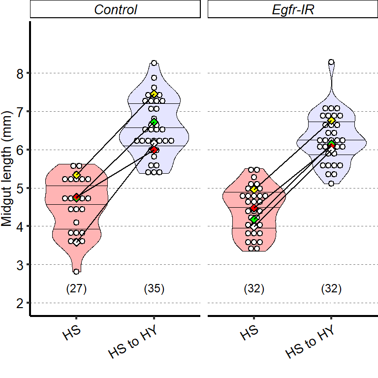
6.1.5 Figure 6F
Insulin signaling with a dominant negative construct in progenitor cells results in less proliferation
tab_PH3_InR =
d[["6F"]]%>%
mutate_at(vars(!starts_with("Total")),as.factor)%>%
dplyr::rename(PH3_positive_cell=Total.PH3,
Day_of_treatment=Day)%>%
as.data.frame()%>%
mutate(Male.Line=fct_relevel(Male.Line,c("wdah","InR-DN")))
Sample_size=
tab_PH3_InR%>%
group_by(Male.Line)%>%
summarise(Sample_size=n())
###Stats
mod.gen = fitme(PH3_positive_cell ~ Male.Line + (1 | Repeat),data = subset(tab_PH3_InR,!is.na(PH3_positive_cell)))
shapiro.test(residuals(mod.gen))
Shapiro-Wilk normality test
data: residuals(mod.gen)
W = 0.87431, p-value = 0.002092bptest(PH3_positive_cell ~ Male.Line + (1 / Repeat),data = subset(tab_PH3_InR,!is.na(PH3_positive_cell)))
studentized Breusch-Pagan test
data: PH3_positive_cell ~ Male.Line + (1/Repeat)
BP = 5.6857, df = 1, p-value = 0.0171mod.gen1 = fitme(PH3_positive_cell ~ 1 + (1 | Repeat),data = subset(tab_PH3_InR,!is.na(PH3_positive_cell)))
test = anova(mod.gen, mod.gen1)
Chi2_LRT_growth = 2*(mod.gen$APHLs[["p_v"]]-mod.gen1$APHLs[["p_v"]])
tab_stat = data.frame(Variable = as.character(paste("Control vs InR-DN")),
Rep = nlevels(tab_PH3_InR$Repeat),
chi2_LR = round(as.numeric(test$basicLRT$chi2_LR), digits = 2),
intercept = format(mod.gen$fixef[1],digits=3),
estimate = format(mod.gen$fixef[2],digits=3),
df = as.numeric(test$basicLRT$df),
Pvalue = as.numeric(format(pchisq(Chi2_LRT_growth,df=1,lower.tail = F),digits=2)))
tab_stat$sig = ifelse(tab_stat$Pvalue < 0.05 & tab_stat$Pvalue > 0.01, "*",
ifelse(tab_stat$Pvalue < 0.01 & tab_stat$Pvalue > 0.001, "**",
ifelse(tab_stat$Pvalue < 0.001, "***", "")))
tab_stat%>%
kable(col.names = c("Comparison", "Replicates", "Chi2","Intercept","Estimate","df" ,"p-value","Signif."),row.names = FALSE) %>% add_header_above(c("PH3_positive_cell ~ Genotype + (1 | Repeat)" = 8))%>%
kable_styling(bootstrap_options = c("striped", "hover", "condensed"), full_width = F)| Comparison | Replicates | Chi2 | Intercept | Estimate | df | p-value | Signif. |
|---|---|---|---|---|---|---|---|
| Control vs InR-DN | 2 | 14 | 6.79 | -5.85 | 1 | 0.00018 | *** |
### Plot
tab_PH3_InR$Female.Line = factor(tab_PH3_InR$Female.Line, labels = c(expression(italic(paste("Es",g^{TS},">",sep="")))))
Plot_Fig6F=
ggplot(tab_PH3_InR, aes(x = Male.Line, y = PH3_positive_cell))+
geom_boxplot(aes(fill = Diet), colour = "black", size = 0.2,outlier.shape = NA) +
geom_dotplot( colour = "black", fill = "white", binaxis = "y", stackdir = "center", binwidth = 0.6) +
geom_text(data = Sample_size, mapping = aes(x = Male.Line, y = -1.2, label = paste("(",Sample_size,")",sep="")),size=3)+
geom_signif(data = tab_stat,aes(xmin = 1, xmax = 2, annotations = formatC(paste("p=",Pvalue), digits = 2), y_position = 16), textsize = 3, vjust = -0.2, manual = TRUE, tip_length = c(0.01, 0.01))+
facet_grid(.~Female.Line, labeller = label_parsed)+
scale_fill_manual(values="#E5E5FF")+
scale_x_discrete("",
limits=c("wdah","InR-DN"),
labels=c("Control","InR-DN"))+
scale_y_continuous(expression(paste("pH3" ^ "+", " cells")),
limits=c(-1.4,21),
breaks=seq(0,20,by=4))+
stat_summary(fun = mean, geom = "point", size = 3, shape = 18, colour = "black", aes(group = Repeat)) +
stat_summary(fun = mean, geom = "point", size = 2, shape = 18, aes(group = Repeat, colour = Repeat)) +
scale_color_manual(values = palette_mean) +
theme(panel.grid.major.y = element_line(colour = grey(0.45), linetype = "dashed", size = 0.2),
panel.background = element_blank(),
axis.title.x = element_text(size=Smallfont,colour="black"),
axis.title.y = element_text(size=Smallfont,colour="black", margin = margin(t = 0, r = -0.15, b = 0, l = 0, unit = "cm")),
axis.line.x = element_line(colour="black",size=0.75),
axis.line.y = element_line(colour="black",size=0.75),
axis.ticks.x = element_line(size = 0.75),
axis.ticks.y = element_line(size = 0.75),
axis.text.x = element_text(size=Smallfont,colour="black",angle=30,hjust=1, face= "italic"),
axis.text.y = element_text(size=Smallfont,colour="black"),
plot.margin = unit(Margin, "cm"),
legend.direction = "vertical",
legend.box = "horizontal",
legend.position = "none",
legend.key.height = unit(0.4, "cm"),
legend.key.width= unit(0.6, "cm"),
legend.title = element_text(face="italic",size=Smallfont),
legend.key = element_rect(colour = 'white', fill = "white", linetype='dashed'),
legend.text = element_text(size=SuperSmallfont),
legend.background = element_rect(fill=NA),
strip.text.x = element_text(size = Smallfont, colour = "black", face = "italic", margin = margin(t = 1, r = 0, b = 1, l = 0)),
strip.text.y = element_text(size = Smallfont, colour = "black", face = "italic", margin = margin(t = 1, r = 0, b = 1, l = 0)),
strip.background = element_rect(fill=NA, colour="black"),
strip.placement="outside")
Plot_Fig6F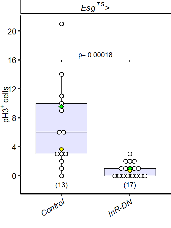
6.1.6 Figure 6G
EsgTS>UAS-InR-DN resulting in the same midgut length growth as the control. Statistical comparison for G is for the interaction between diet and genotype.
tab_length_InDN =
subset(d[["6G"]],Diet%in%c("HS D0","HStoHY D7"))%>%
mutate_at(vars(!starts_with("Total")),as.factor)%>%
mutate(Total_Length_mm=Total.L/1000)%>%
dplyr::rename(Day_of_treatment=Day,
Female_Line=Female.Line,
Male_Line=Male.Line)%>%
as.data.frame()%>%
mutate(Male_Line=fct_relevel(Male_Line,c("Control","InR-DN")))
Sample_size=
tab_length_InDN%>%
group_by(Diet,Male_Line)%>%
summarise(Sample_size=n())
###Stats
mod.gen = fitme(log(Total_Length_mm) ~ Diet * Male_Line + (1 | PhaseRep),data = tab_length_InDN)
shapiro.test(residuals(mod.gen))
Shapiro-Wilk normality test
data: residuals(mod.gen)
W = 0.9894, p-value = 0.1608bptest(log(Total_Length_mm) ~ Diet + Male_Line + (1 / PhaseRep),data = tab_length_InDN)
studentized Breusch-Pagan test
data: log(Total_Length_mm) ~ Diet + Male_Line + (1/PhaseRep)
BP = 3.8117, df = 2, p-value = 0.1487mod.gen1 = fitme(log(Total_Length_mm) ~ Diet + Male_Line + (1 | PhaseRep),data = tab_length_InDN)
test = anova(mod.gen, mod.gen1)
Chi2_LRT_growth = 2*(mod.gen$APHLs[["p_v"]]-mod.gen1$APHLs[["p_v"]])
tab_stat = data.frame(Variable = as.character(paste("Control vs InR-DN")),
Rep = nlevels(tab_PH3_esg$Repeat),
chi2_LR = round(as.numeric(test$basicLRT$chi2_LR), digits = 2),
intercept = format(mod.gen$fixef[1],digits=3),
estimate = format(mod.gen$fixef[2],digits=3),
df = as.numeric(test$basicLRT$df),
Pvalue = as.numeric(format(pchisq(Chi2_LRT_growth,df=1,lower.tail = F),digits=2)))
tab_stat$sig = ifelse(tab_stat$Pvalue < 0.05 & tab_stat$Pvalue > 0.01, "*",
ifelse(tab_stat$Pvalue < 0.01 & tab_stat$Pvalue > 0.001, "**",
ifelse(tab_stat$Pvalue < 0.001, "***", "")))
tab_stat%>%
kable(col.names = c("Comparison", "Replicates", "Chi2","Intercept","Estimate","df" ,"p-value","Signif."),row.names = FALSE) %>% add_header_above(c("log(Total_length_mm) ~ Diet + Genotype + Diet : Genotype + (1 | Repeat)" = 8))%>%
kable_styling(bootstrap_options = c("striped", "hover", "condensed"), full_width = F)| Comparison | Replicates | Chi2 | Intercept | Estimate | df | p-value | Signif. |
|---|---|---|---|---|---|---|---|
| Control vs InR-DN | 2 | 0.01 | 1.53 | 0.249 | 1 | 0.92 |
tab_stat$Male_Line="InR-DN"
tab_stat6G = tab_stat
### Plot
tab_length_InDN$Male_Line = factor(tab_length_InDN$Male_Line, labels = c("Control","InR-DN"))
Sample_size$Male_Line = factor(Sample_size$Male_Line, labels = c("Control","InR-DN"))
Plot_Fig6G=
ggplot(tab_length_InDN, aes(x = Diet, y = Total_Length_mm))+
geom_violin(aes(fill = Diet), draw_quantiles = c(0.25, 0.5, 0.75), colour = "black", size = 0.2,adjust = 0.8) +
geom_dotplot( colour = "black", fill = "white", binaxis = "y", stackdir = "center", binwidth = 0.15) +
geom_text(data = Sample_size, mapping = aes(x = Diet, y = 2.5, label = paste("(",Sample_size,")",sep="")),size=3)+
facet_grid(.~Male_Line)+
scale_fill_manual(values=cbbHS_HStoHY)+
scale_x_discrete("",
limits=c("HS D0","HStoHY D7"),
labels=c("HS","HS to HY"))+
scale_y_continuous("Midgut length (mm)",
limits=c(2,9),
breaks=seq(2,8,by=1))+
stat_summary(fun = mean, geom = "point", size = 3, shape = 18, colour = "black", aes(group = Repeat)) +
stat_summary(fun = mean, geom = "point", size = 2, shape = 18, aes(group = Repeat, colour = Repeat)) +
stat_summary(fun = mean, colour = "black", geom = "line", aes(group = Repeat)) +
scale_color_manual(values = palette_mean) +
theme(panel.grid.major.y = element_line(colour = grey(0.45), linetype = "dashed", size = 0.2),
panel.background = element_blank(),
axis.title.x = element_text(size=Smallfont,colour="black"),
axis.title.y = element_text(size=Smallfont,colour="black"),
axis.line.x = element_line(colour="black",size=0.75),
axis.line.y = element_line(colour="black",size=0.75),
axis.ticks.x = element_line(size = 0.75),
axis.ticks.y = element_line(size = 0.75),
axis.text.x = element_text(size=Smallfont,colour="black",angle=30,hjust=1),
axis.text.y = element_text(size=Smallfont,colour="black"),
plot.margin = unit(Margin, "cm"),
legend.direction = "vertical",
legend.box = "horizontal",
legend.position = "none",
legend.key.height = unit(0.4, "cm"),
legend.key.width= unit(0.6, "cm"),
legend.title = element_text(face="italic",size=Smallfont),
legend.key = element_rect(colour = 'white', fill = "white", linetype='dashed'),
legend.text = element_text(size=SuperSmallfont),
legend.background = element_rect(fill=NA),
strip.text.x = element_text(size = Smallfont, colour = "black", face="italic", margin = margin(t = 2, r = 0, b = 2, l = 0)),
strip.text.y = element_text(size = Smallfont, colour = "black", margin = margin(t = 2, r = 0, b = 2, l = 0)),
strip.background = element_rect(fill=NA, colour="black"),
strip.placement="outside")
Plot_Fig6G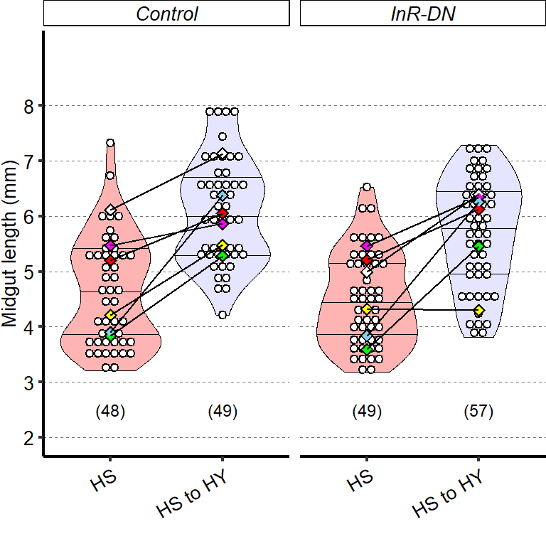
6.1.7 Figure 6H-I
Increase in midgut length despite proliferation blockage is accompanied with compensatory area increase of EC. Representative pictures of midguts stained with membrane marker Mesh (white), shifted from HS to HY for 7 days show bigger cells on EsgTS>UAS-Egfr-IR (I, right) compared to control (H, left). Complete graphical annotation can be found in manuscript figures
img = readImage("F:/Dropbox/Github/Bonfini_eLife_2021/data/6H.jpg")
gob_imageFig6H = rasterGrob(img)
grid.draw(gob_imageFig6H)
img = readImage("F:/Dropbox/Github/Bonfini_eLife_2021/data/6I.jpg")
gob_imageFig6I = rasterGrob(img)
grid.draw(gob_imageFig6I)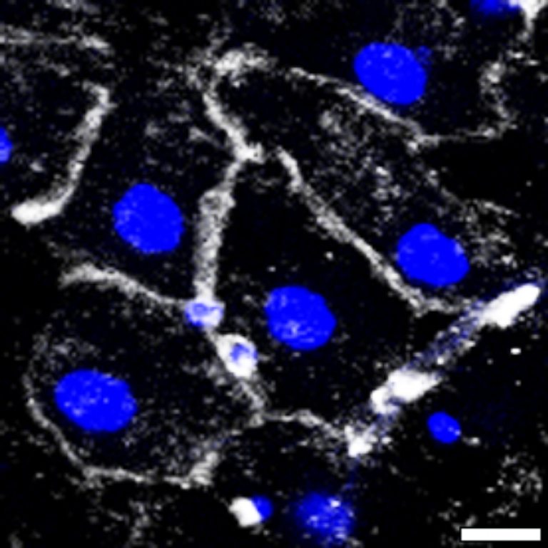
6.1.8 Figure 6J
Quantification of EC cell size shows compensatory effect in ECs of EsgTS>Egfr-IR.Statistical comparison is for the interaction between diet and genotype.
tab_area_esg =
subset(d[["6J"]],Area<=1300)%>%
mutate_at(vars(!starts_with("Area")),as.factor)%>%
dplyr::rename(Day_of_treatment=Day,
Female_Line=Female.Line,
Male_Line=Male.Line)%>%
as.data.frame()%>%
mutate(Diet=fct_relevel(Diet,c("HS", "HStoHY")))
Sample_size=
tab_area_esg%>%
group_by(Diet,Male_Line)%>%
summarise(Sample_size=n())
###Stats
# D7
mod.gen = fitme(log(Area) ~ Diet * Male_Line + (1 | Repeat) ,data = tab_area_esg)
shapiro.test(residuals(mod.gen))
Shapiro-Wilk normality test
data: residuals(mod.gen)
W = 0.99806, p-value = 0.06875bptest(log(Area) ~ Diet * Male_Line+ (1 / Repeat) ,data = tab_area_esg)
studentized Breusch-Pagan test
data: log(Area) ~ Diet * Male_Line + (1/Repeat)
BP = 6.8989, df = 3, p-value = 0.07519mod.gen1 = fitme(log(Area) ~ Diet + Male_Line + (1 | Repeat),data = tab_area_esg)
test = anova(mod.gen, mod.gen1)
Chi2_LRT_growth = 2*(mod.gen$APHLs[["p_v"]]-mod.gen1$APHLs[["p_v"]])
tab_stat = data.frame(Variable = as.character(paste("Response Control vs Egfr")),
Rep = nlevels(tab_area_esg$Repeat),
chi2_LR = round(as.numeric(test$basicLRT$chi2_LR), digits = 2),
intercept = format(mod.gen$fixef[1],digits=3),
estimate = format(mod.gen$fixef[4],digits=3),
df = as.numeric(test$basicLRT$df),
Pvalue = as.numeric(format(pchisq(Chi2_LRT_growth,df=1,lower.tail = F),digits=2)))
tab_stat$sig = ifelse(tab_stat$Pvalue < 0.05 & tab_stat$Pvalue > 0.01, "*",
ifelse(tab_stat$Pvalue < 0.01 & tab_stat$Pvalue > 0.001, "**",
ifelse(tab_stat$Pvalue < 0.001, "***", "")))
tab_stat%>%
kable(col.names = c("Variable", "Replicates", "Chi2","Intercept","Estimate","df" ,"p-value","Signif."),row.names = FALSE) %>% add_header_above(c("log(Cell area) ~ Diet + Genotype + Diet : Genotype + (1 | Repeat)" = 8))%>%
kable_styling(bootstrap_options = c("striped", "hover", "condensed"), full_width = F)| Variable | Replicates | Chi2 | Intercept | Estimate | df | p-value | Signif. |
|---|---|---|---|---|---|---|---|
| Response Control vs Egfr | 2 | 10.51 | 4.49 | 0.132 | 1 | 0.0012 | ** |
tab_stat_6J=tab_stat
tab_stat_6J$Male_Line="Egfr-IR"
tab_stat_6J$Diet=c("HStoHY")
tab_stat_6J$yposition = c(0.6)
tab_stat_6J$xposition = c(1.5)
### Plot
z = max(tab_area_esg$Area/1000, na.rm = TRUE)
Plot_Fig6J=
ggplot(tab_area_esg, aes(x = Diet, y = Area/1000))+
geom_violin(aes(fill = C.G), draw_quantiles = c(0.25, 0.5, 0.75), colour = "black", size = 0.2,adjust = 2) +
geom_dotplot( colour = "black", fill = "white", binaxis = "y", stackdir = "center", binwidth = z/120) +
geom_text(data = Sample_size, mapping = aes(x = Diet, y = -0.1, label = paste("(",Sample_size,")",sep="")),size=3)+
facet_grid(.~Male_Line)+
scale_fill_manual(values=cbbHS_HStoHY)+
scale_x_discrete("",
limits=c("HS","HStoHY"),
labels=c("HS","HS to HY"))+
scale_y_continuous(expression(paste("EC area (10"^3, "mm"^2,")",sep="")),
limits=c(-0.1,1.1),
breaks=seq(0,1.1,by=0.4))+
stat_summary(fun = mean, geom = "point", size = 3, shape = 18, colour = "black", aes(group = Repeat)) +
stat_summary(fun = mean, geom = "point", size = 2, shape = 18, aes(group = Repeat, colour = Repeat)) +
stat_summary(fun = mean, colour = "black", geom = "line", aes(group = Repeat)) +
scale_color_manual(values = palette_mean) +
theme(panel.grid.major.y = element_line(colour = grey(0.45), linetype = "dashed", size = 0.2),
panel.background = element_blank(),
axis.title.x = element_text(size=Smallfont,colour="black"),
axis.title.y = element_text(size=Smallfont,colour="black"),
axis.line.x = element_line(colour="black",size=0.75),
axis.line.y = element_line(colour="black",size=0.75),
axis.ticks.x = element_line(size = 0.75),
axis.ticks.y = element_line(size = 0.75),
axis.text.x = element_text(size=Smallfont,colour="black",angle=30,hjust=1),
axis.text.y = element_text(size=Smallfont,colour="black"),
plot.margin = unit(margin(0, 0, 0, 0, unit = "cm")),
legend.direction = "vertical",
legend.box = "horizontal",
legend.position = "none",
legend.key.height = unit(0.4, "cm"),
legend.key.width= unit(0.6, "cm"),
legend.title = element_text(face="italic",size=Smallfont),
legend.key = element_rect(colour = 'white', fill = "white", linetype='dashed'),
legend.text = element_text(size=SuperSmallfont),
legend.background = element_rect(fill=NA),
strip.text = element_text(size =Smallfont, colour = "black",face="italic", margin = margin(t = 2, r = 0, b = 2, l = 0)),
strip.background = element_rect(fill=NA, colour="black"),
strip.placement="outside")
Plot_Fig6J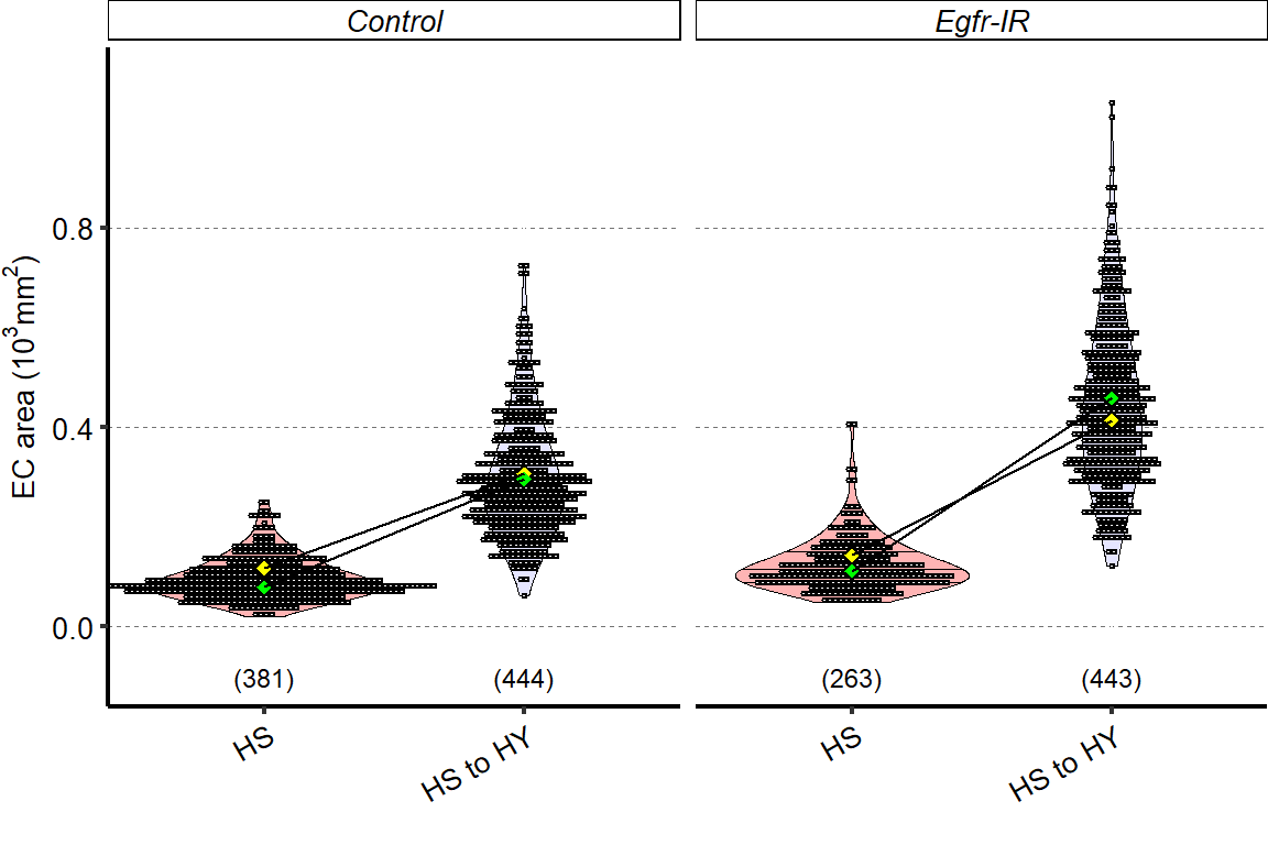
##Export Figure 6
6.2 Figure 6 - supplementary 1
6.2.1 Figure 6S1A
Changes in the number of pH3+ cells between HS and HY (ratio HY/HS of mean pH3+ cells) does not correlate with changes in midgut size between HS and HY (ratio HY/HS of mean midgut length) across selected DGRP lines.
tab_corr_length_cell_DGRP_mean_ph3 =
tab_corr_length_cell_DGRP%>%
group_by(ral,diet)%>%
summarise(mean_ph3=mean(ph3,na.rm=T))%>%
spread(diet,mean_ph3)%>%
dplyr::rename(Mean_ph3_HS=HS,
Mean_ph3_HY=HY)%>%
mutate(Ratio_ph3 = Mean_ph3_HY/Mean_ph3_HS)
tab_corr_length_cell_DGRP_mean_length =
tab_corr_length_cell_DGRP%>%
group_by(ral,diet)%>%
summarise(mean_length=mean(len,na.rm=T))%>%
spread(diet,mean_length)%>%
dplyr::rename(mean_length_HS=HS,
mean_length_HY=HY)%>%
mutate(Ratio_length = mean_length_HY/mean_length_HS)
tab_corr_length_cell_DGRP_mean= left_join(tab_corr_length_cell_DGRP_mean_length,tab_corr_length_cell_DGRP_mean_ph3)
tab_corr_length_cell_DGRP_mean=as.data.frame(tab_corr_length_cell_DGRP_mean)
test =
with(tab_corr_length_cell_DGRP_mean,
cor.test(Ratio_ph3,Ratio_length,method="pearson"))
tab_stat = data.frame(Statistic = test$statistic,
cor = test$estimate,
Pvalue = test$p.value)
levels(tab_corr_length_cell_DGRP_mean$ral) <- c("Ral 356", "Ral 362", "Ral 370", "Ral 502", "Ral 765", "Ral 853", "Ral 911" )
Plot_Fig6S1A =
ggplot(tab_corr_length_cell_DGRP_mean,aes(x=Ratio_ph3,y=Ratio_length,label=ral))+
geom_point()+
scale_x_continuous(expression(paste("Ratio HY/HS (mean pH3" ^ "+", " cells)")),
limits=c(0.8,1.8),
breaks=c(seq(0.8,2.8,by=0.1)))+
scale_y_continuous("Ratio HY/HS (mean midgut length)",
limits=c(0.8,1.8),
breaks=c(seq(0.8,2.8,by=0.2)))+
geom_text_repel(data=tab_corr_length_cell_DGRP_mean,size=3)+
geom_smooth(method="lm")+
geom_text(data = tab_stat, mapping = aes(x = 1.6, y = 1.7, label = paste("cor=", format(cor, digits=2), "p=",format(Pvalue,digits=2))),size=3)+ theme(panel.grid.major.y = element_line(colour = grey(0.45), linetype = "dashed", size = 0.2),
panel.background = element_blank(),
(panel.border = element_blank()),
axis.title.x = element_text(size=Smallfont,colour="black"),
axis.title.y = element_text(size=Smallfont,colour="black"),
axis.line.x = element_line(colour="black",size=0.75),
axis.line.y = element_line(colour="black",size=0.75),
axis.ticks.x = element_blank(),
axis.ticks.y = element_line(size = 0.75),
axis.text.x = element_text(size=Smallfont,colour="black"),
axis.text.y = element_text(size=Smallfont,colour="black"),
plot.margin = unit(Margin, "cm"),
legend.direction = "horizontal",
legend.box = "horizontal",
legend.position = c(0.25,0.98),
legend.key.height = unit(0.4, "cm"),
legend.key.width= unit(0.4, "cm"),
legend.title = element_blank(),
legend.key = element_rect(colour = 'white', fill = "white", linetype='dashed'),
legend.text = element_text(size=Smallfont),
legend.background = element_rect(fill=NA))+
guides(color=guide_legend(ncol=3))
Plot_Fig6S1A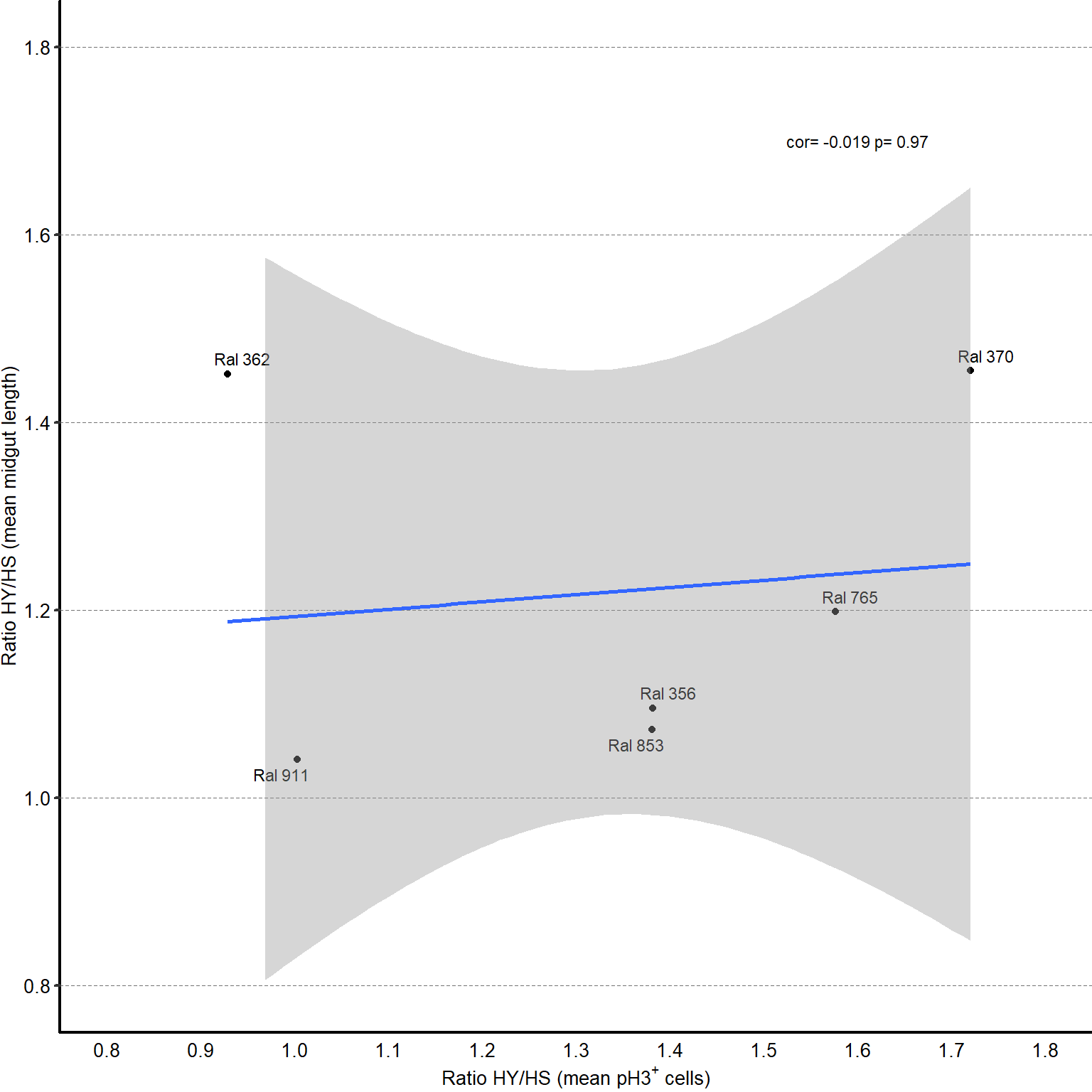
6.2.2 Figure 6S1B-E
Overexpression of reaper in progenitor cells (marked in red) via EsgTS>rpr-OE results in loss of marked progenitor cells (C) compared to control (B) in region 4 of midguts, after 12 days post eclosion on HS diet (7 days at 29°C with TARGET system active). Shifting the flies on HY for additional 7 days results in a change in morphology on midguts overexpressing reaper, reminiscent of EsgTS>UAS-Egfr-IR midguts .Complete graphical annotation can be found in manuscript figures
img = readImage("F:/Dropbox/Github/Bonfini_eLife_2021/data/6 - S1B.jpg")
gob_imageFig6S1B = rasterGrob(img)
grid.draw(gob_imageFig6S1B)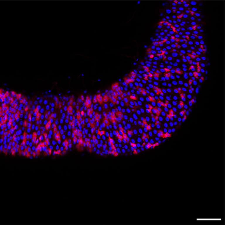
img = readImage("F:/Dropbox/Github/Bonfini_eLife_2021/data/6 - S1C.jpg")
gob_imageFig6S1C = rasterGrob(img)
grid.draw(gob_imageFig6S1C)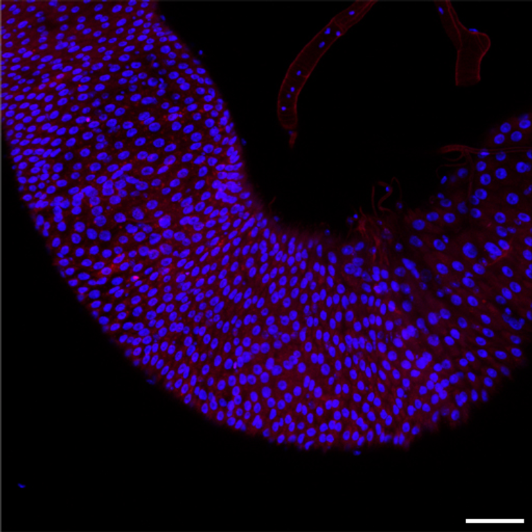
img = readImage("F:/Dropbox/Github/Bonfini_eLife_2021/data/6 - S1D.jpg")
gob_imageFig6S1D = rasterGrob(img)
grid.draw(gob_imageFig6S1D)
img = readImage("F:/Dropbox/Github/Bonfini_eLife_2021/data/6 - S1E.jpg")
gob_imageFig6S1E = rasterGrob(img)
grid.draw(gob_imageFig6S1E)
6.2.3 Figure 6S1F
EsgTS> rpr-OE midguts are still able to reach a similar length to controls .Complete graphical annotation can be found in manuscript figures
tab_length_rpr =
d[["6 - S1F"]]%>%
mutate_at(vars(!starts_with("Total")),as.factor)%>%
mutate(Total_Length_mm=Total.L/1000)%>%
dplyr::rename(Day_of_treatment=Day,
Female_Line=Female.Line,
Male_Line=Male.Line)%>%
as.data.frame()%>%
mutate(Male_Line=fct_relevel(Male_Line, "Control", "rpr-OE"))
Sample_size=
tab_length_rpr%>%
group_by(Diet, Male_Line)%>%
summarise(Sample_size=n())
###Stats
mod.gen = fitme(log(Total_Length_mm) ~ Diet * Male_Line + (1 | Repeat),data = tab_length_rpr)
shapiro.test(residuals(mod.gen))
Shapiro-Wilk normality test
data: residuals(mod.gen)
W = 0.97478, p-value = 0.08696bptest(log(Total_Length_mm) ~ Diet + Male_Line + (1 / Repeat),data = tab_length_rpr)
studentized Breusch-Pagan test
data: log(Total_Length_mm) ~ Diet + Male_Line + (1/Repeat)
BP = 5.6339, df = 2, p-value = 0.05979mod.gen1 = fitme(log(Total_Length_mm) ~ Diet + Male_Line + (1 | Repeat),data = tab_length_rpr)
test = anova(mod.gen, mod.gen1)
test chi2_LR df p_value
p_v 1.128544 1 0.2880861Chi2_LRT_growth = 2*(mod.gen$APHLs[["p_v"]]-mod.gen1$APHLs[["p_v"]])
tab_stat = data.frame(Comparison = as.character(paste("Interaction Control vs Interaction Rpr-OE")),
Male_Line = as.character(paste("rpr-OE")),
Rep = nlevels(tmp$Repeat),
chi2_LR = round(as.numeric(test$basicLRT$chi2_LR), digits = 2),
intercept = format(mod.gen$fixef[1],digits=3),
estimate = format(mod.gen$fixef[2],digits=3),
df = as.numeric(test$basicLRT$df),
Pvalue = as.numeric(format(pchisq(Chi2_LRT_growth,df=1,lower.tail = F),digits=1,scientific=F)))
tab_stat$sig = ifelse(tab_stat$Pvalue < 0.05 & tab_stat$Pvalue > 0.01, "*",
ifelse(tab_stat$Pvalue < 0.01 & tab_stat$Pvalue > 0.001, "**",
ifelse(tab_stat$Pvalue < 0.001, "***", "")))
tab_stat_rpr=tab_stat
tab_stat_rpr%>%
kable(col.names = c("Comparison", "Variable", "Replicates", "Chi2","Intercept","Estimate","df" ,"p-value","Signif."),row.names = FALSE) %>%
add_header_above(c("log(Total_Length_mm) ~ Diet + Genotype + Diet : Genotype + (1 | Repeat)" = 9))%>%
kable_styling(bootstrap_options = c("striped", "hover", "condensed"), full_width = F)| Comparison | Variable | Replicates | Chi2 | Intercept | Estimate | df | p-value | Signif. |
|---|---|---|---|---|---|---|---|---|
| Interaction Control vs Interaction Rpr-OE | rpr-OE | 0 | 1.13 | 1.53 | 0.278 | 1 | 0.3 |
### Plot
z = max(tab_length_rpr$Total_Length_mm, na.rm = TRUE)
Plot_Fig6S1F=
ggplot(tab_length_rpr, aes(x = Diet, y = Total_Length_mm))+
geom_violin(aes(fill = Diet), draw_quantiles = c(0.25, 0.5, 0.75), colour = "black", size = 0.2,adjust = 0.8) +
geom_dotplot( colour = "black", fill = "white", binaxis = "y", stackdir = "center", binwidth = z/40) +
geom_text(data = Sample_size, mapping = aes(x = Diet, y = 2.5, label = paste("(",Sample_size,")",sep="")),size=3)+
facet_grid(.~Male_Line )+
scale_fill_manual(values=cbbHS_HStoHY)+
scale_x_discrete("",
limits=c("HS","HStoHY"),
labels=c("HS","HS to HY"))+
scale_y_continuous("Midgut length (mm)",
limits=c(2,9),
breaks=seq(2,8,by=1))+
stat_summary(fun = mean, geom = "point", size = 3, shape = 18, colour = "black", aes(group = Repeat)) +
stat_summary(fun = mean, geom = "point", size = 2, shape = 18, aes(group = Repeat, colour = Repeat)) +
stat_summary(fun = mean, colour = "black", geom = "line", aes(group = Repeat)) +
scale_color_manual(values = palette_mean) +
theme(panel.grid.major.y = element_line(colour = grey(0.45), linetype = "dashed", size = 0.2),
panel.background = element_blank(),
axis.title.x = element_text(size=Smallfont,colour="black"),
axis.title.y = element_text(size=Smallfont,colour="black"),
axis.line.x = element_line(colour="black",size=0.75),
axis.line.y = element_line(colour="black",size=0.75),
axis.ticks.x = element_line(size = 0.75),
axis.ticks.y = element_line(size = 0.75),
axis.text.x = element_text(size=Smallfont,colour="black",angle=30,hjust=1),
axis.text.y = element_text(size=Smallfont,colour="black"),
plot.margin = unit(Margin, "cm"),
legend.direction = "vertical",
legend.box = "horizontal",
legend.position = "none",
legend.key.height = unit(0.4, "cm"),
legend.key.width= unit(0.6, "cm"),
legend.title = element_text(face="italic",size=Smallfont),
legend.key = element_rect(colour = 'white', fill = "white", linetype='dashed'),
legend.text = element_text(size=SuperSmallfont),
legend.background = element_rect(fill=NA),
strip.text.x = element_text(size = xSmallfont, colour = "black", angle=0, face = "italic", margin = margin(t = 2, r = 0, b = 2, l = 0)),
strip.text.y = element_text(size = xSmallfont, colour = "black", angle=0, face = "italic", margin = margin(t = 2, r = 0, b = 2, l = 0)),
strip.background = element_rect(fill=NA, colour="black"),
strip.placement="outside")
Plot_Fig6S1F
##Export Figure 6 - supplementary 1
7 Figure 7. Enterocyte resizing is required for midgut plasticity
7.1 Figure 7 - main
7.1.1 Figure 7A
Enterocyte size mostly correlates with midgut length. Quantification of EC area across a selected panel of DGRP lines comprising high and low responder shows that midgut length mostly correlates with EC cell area. Lines on plot show smoothed splines.
wolb = d[["DGRP_wolbachia_DFD"]]
colnames(wolb) = c("dgrp.id", "wolbachia")
wolb$dgrp.id = gsub("line_", "", wolb$dgrp.id)
tab_corr_length_cell_DGRP = subset(d[["6A - 7A"]])
tab_corr_length_cell_DGRP = merge(tab_corr_length_cell_DGRP, wolb, by.x="DGRP.number", by.y="dgrp.id", all.x=T, all.y=F)
colnames(tab_corr_length_cell_DGRP) = tolower(colnames(tab_corr_length_cell_DGRP))
colnames(tab_corr_length_cell_DGRP)[3] = "repl"
tab_corr_length_cell_DGRP=
tab_corr_length_cell_DGRP%>%
dplyr::rename(ral=dgrp.number,
len=total.l,
ph3=total.ph3,
ec.area=area)%>%
mutate(ral=paste("Ral",ral,sep="_"))%>%
mutate_if(is.character,as.factor)
gut_mean=
tab_corr_length_cell_DGRP %>%
group_by(ral, diet,cross,gutnumber)%>%
summarize(mean_gut_len=mean(len,na.rm=T),
mean_cell_size=mean(ec.area,na.rm=T),
se_cell_size=sd(ec.area,na.rm=T)/ sqrt(length(ec.area[!is.na(ec.area)])),
mean_PH3=mean(ph3,na.rm=T)) %>%
mutate(Group=paste(cross,gutnumber,sep="_"))Error: Problem with `summarise()` column `se_cell_size`.
i `se_cell_size = sd(ec.area, na.rm = T)/sqrt(length(ec.area[!is.na(ec.area)]))`.
x argument inutilisé (na.rm = T)
i The error occurred in group 1: ral = Ral_356, diet = HS, cross = 4 R1, gutnumber = 1.levels(gut_mean$ral) <- c("Ral 356", "Ral 362", "Ral 370", "Ral 502", "Ral 765", "Ral 853", "Ral 911" )
gut_mean$ral <- factor(gut_mean$ral, levels = c("Ral 356", "Ral 502", "Ral 765", "Ral 853", "Ral 911", "Ral 362", "Ral 370"))
Sample_size=
gut_mean%>%
group_by(diet, ral)%>%
summarise(Sample_size=n())%>%
as.data.frame()%>%
mutate(ral=fct_relevel(ral,"Ral 356", "Ral 502", "Ral 765", "Ral 853", "Ral 911", "Ral 362", "Ral 370"))
# stat over all
mod.gen = fitme(log10(I(mean_gut_len/1000)) ~ mean_cell_size + (1 | ral),data = gut_mean)
shapiro.test(residuals(mod.gen))
Shapiro-Wilk normality test
data: residuals(mod.gen)
W = 0.99351, p-value = 0.3142bptest(log10(I(mean_gut_len/1000)) ~ mean_cell_size + (1 / ral),data = gut_mean)
studentized Breusch-Pagan test
data: log10(I(mean_gut_len/1000)) ~ mean_cell_size + (1/ral)
BP = 0.26958, df = 1, p-value = 0.6036mod.gen1 = fitme(log10(I(mean_gut_len/1000)) ~ 1 + (1 | ral),data =gut_mean)
test = anova(mod.gen, mod.gen1)
Chi2_LRT_growth = 2*(mod.gen$APHLs[["p_v"]]-mod.gen1$APHLs[["p_v"]])
tab_stat = data.frame(Variable = as.character(paste("Cell area")),
Number_genotypes = nlevels(gut_mean$ral),
chi2_LR = round(as.numeric(test$basicLRT$chi2_LR), digits = 2),
intercept = format(mod.gen$fixef[1],digits=3),
estimate = format(mod.gen$fixef[2],digits=3),
df = as.numeric(test$basicLRT$df),
Pvalue = as.numeric(format(pchisq(Chi2_LRT_growth,df=1,lower.tail = F),digits=2)))
#stat per line
Cor_area=NULL
for(i in unique(gut_mean$ral)){
# print(i)
Cor_area_HS=
with(subset(gut_mean,ral==i& diet=="HS"),
cor.test(log(mean_gut_len,2),mean_cell_size))
Cor_area_HY=
with(subset(gut_mean,ral==i& diet=="HY"),
cor.test(log(mean_gut_len,2),mean_cell_size))
Cor_area_tmp = data.frame(ral = as.character(i),
diet=c("HS","HY"),
Cor = c(format(as.numeric(Cor_area_HS$estimate), digits = 2),format(as.numeric(Cor_area_HY$estimate), digits = 2)),
Pvalue = c(format(as.numeric(Cor_area_HS$p.value), digits = 2),format(as.numeric(Cor_area_HY$p.value), digits = 2)))
Cor_area= rbind(Cor_area,Cor_area_tmp)
}
Cor_area$padj=p.adjust(Cor_area$Pvalue,method = "BH")
Cor_area$sig= ifelse(Cor_area$padj < 0.05 & Cor_area$padj > 0.01, "*",
ifelse(Cor_area$padj < 0.01 & Cor_area$padj > 0.001, "**",
ifelse(Cor_area$padj < 0.001, "***", "ns")))
tmp=subset(gut_mean,diet=="HS")
stat_position_HS = aggregate(data=tmp,mean_gut_len/1000 ~ ral, max)
stat_position_HS$diet="HS"
tmp=subset(gut_mean,diet=="HY")
stat_position_HY = aggregate(data=tmp,mean_gut_len/1000 ~ ral, max)
stat_position_HY$diet="HY"
stat_position=rbind(stat_position_HS,stat_position_HY)
colnames(stat_position)[2]="Stat_position"
Cor_area = left_join(Cor_area,stat_position)
gut_mean$ral <- factor(gut_mean$ral, levels = c("Ral 356", "Ral 502", "Ral 765", "Ral 853", "Ral 911", "Ral 362", "Ral 370"))
Cor_area$ral <- factor(Cor_area$ral, levels = c("Ral 356", "Ral 502", "Ral 765", "Ral 853", "Ral 911", "Ral 362", "Ral 370"))
Plot_Fig7A=
ggplot(gut_mean,aes(x=log2(mean_cell_size), y=mean_gut_len/1000,group=ral))+
geom_point( aes(color=diet,fill=diet),shape=21,size=0.9)+
geom_text(data = Sample_size, mapping = aes(x = 8, y = 2.5, label = paste("(",Sample_size,")",sep="")),size=3)+
geom_text(data = Cor_area, mapping = aes( x=7,y=7,label = sig),size=3)+
facet_grid(ral~diet)+
scale_y_continuous("Midgut length (mm)")+
scale_x_continuous(expression(paste("Cell size (", log[2],"(mean\u00B1se))")))+
scale_color_manual("",
limits=c("HS","HY"),
values=palette_diet_2)+
scale_fill_manual("",
limits=c("HS","HY"),
values=palette_diet_2)+
geom_smooth(method="lm",color="black",size=0.5)+
theme(panel.grid.major.y = element_line(colour = grey(0.45), linetype = "dashed", size = 0.2),
panel.background = element_blank(),
axis.title.x = element_text(size=Smallfont,colour="black"),
axis.title.y = element_text(size=Smallfont,colour="black"),
axis.line.x = element_line(colour="black",size=0.75),
axis.line.y = element_line(colour="black",size=0.75),
axis.ticks.x = element_line(size = 0.75),
axis.ticks.y = element_line(size = 0.75),
axis.text.x = element_text(size=Smallfont,colour="black"),
axis.text.y = element_text(size=Smallfont,colour="black"),
plot.margin = unit(Margin, "cm"),
legend.direction = "vertical",
legend.box = "horizontal",
legend.position = "none",
legend.key.height = unit(0.4, "cm"),
legend.key.width= unit(0.6, "cm"),
legend.title = element_text(face="italic",size=Smallfont),
legend.key = element_rect(colour = 'white', fill = "white", linetype='dashed'),
legend.text = element_text(size=SuperSmallfont),
legend.background = element_rect(fill=NA),
strip.text.x = element_text(size = Smallfont, colour = "black", margin = margin(t = 2, r = 0, b = 2, l = 0)),
strip.text.y = element_text(size = Smallfont, colour = "black", face = "italic", margin = margin(t = 2, r = 0, b = 2, l = 0)),
strip.background = element_rect(fill=NA, colour="black"),
strip.placement="outside")
Plot_Fig7A
7.1.2 Figure 7B-C-D
Representative pictures of single cell clones (hsFlp; Act>STOP>Gal4, UAS-GFP) suggest that compared to GFP- cells, TOR downregulation (UAS-Tor-IR, GFP+) results in smaller cells, while TOR hyperactivity (UAS-Rheb-OE, C) increases cell size. Quantification of clone size in D. Single cell clones are marked with GFP (green). Complete graphical annotation can be found in manuscript figures
img = readImage("F:/Dropbox/Github/Bonfini_eLife_2021/data/7B.jpg")
gob_imageFig7B = rasterGrob(img)
grid.draw(gob_imageFig7B)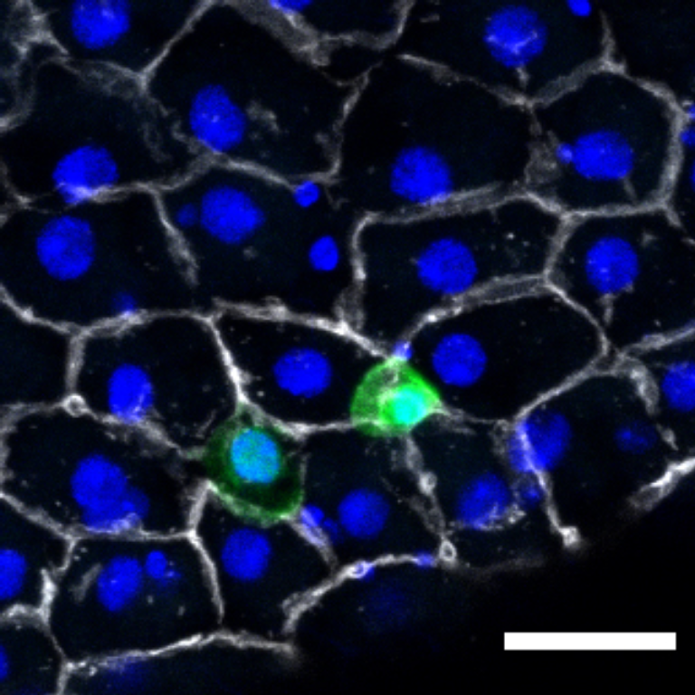
img = readImage("F:/Dropbox/Github/Bonfini_eLife_2021/data/7C.jpg")
gob_imageFig7C = rasterGrob(img)
grid.draw(gob_imageFig7C)
tab_ECclone_quant =
d[["7D"]]%>%
mutate_at(vars(!starts_with("Area")),as.factor)%>%
dplyr::rename(Male_Line=Male.Line)%>%
as.data.frame()%>%
mutate(Male_Line=fct_relevel(Male_Line,"Tor-IR","Rheb-OE"))
Sample_size=
tab_ECclone_quant%>%
group_by(Male_Line, GFP)%>%
summarise(Sample_size=n())%>%
as.data.frame()%>%
mutate(Male_Line=fct_relevel(Male_Line,"Tor-IR","Rheb-OE"))
###Stats
#Tor-IR stats
mod.gen = fitme(log(Area) ~ GFP,data = subset(tab_ECclone_quant, Male_Line=="Tor-IR"))
shapiro.test(residuals(mod.gen))
Shapiro-Wilk normality test
data: residuals(mod.gen)
W = 0.9451, p-value = 1.023e-07bptest(log(Area) ~ GFP ,data = subset(tab_ECclone_quant, Male_Line=="Tor-IR"))
studentized Breusch-Pagan test
data: log(Area) ~ GFP
BP = 0.17945, df = 1, p-value = 0.6718mod.gen1 = fitme(log(Area) ~ 1 ,data = subset(tab_ECclone_quant, Male_Line=="Tor-IR"))
test = anova(mod.gen, mod.gen1)
Chi2_LRT_growth = 2*(mod.gen$APHLs[["p_v"]]-mod.gen1$APHLs[["p_v"]])
tab_stat = data.frame(Variable = as.character(paste("GFP Negative vs Positive (Tor-IR)")),
chi2_LR = round(as.numeric(test$basicLRT$chi2_LR), digits = 2),
intercept = format(mod.gen$fixef[1],digits=3),
estimate = format(mod.gen$fixef[2],digits=3),
df = as.numeric(test$basicLRT$df),
Pvalue = as.numeric(format(pchisq(Chi2_LRT_growth,df=1,lower.tail = F),digits=2)))
tab_stat_TorEC = tab_stat
mod.gen = fitme(log(Area) ~ GFP,data = subset(tab_ECclone_quant, Male_Line=="Rheb-OE"))
shapiro.test(residuals(mod.gen))
Shapiro-Wilk normality test
data: residuals(mod.gen)
W = 0.98578, p-value = 0.01348bptest(log(Area) ~ GFP ,data = subset(tab_ECclone_quant, Male_Line=="Rheb-OE"))
studentized Breusch-Pagan test
data: log(Area) ~ GFP
BP = 0.5099, df = 1, p-value = 0.4752mod.gen1 = fitme(log(Area) ~ 1 ,data = subset(tab_ECclone_quant, Male_Line=="Rheb-OE"))
test = anova(mod.gen, mod.gen1)
Chi2_LRT_growth = 2*(mod.gen$APHLs[["p_v"]]-mod.gen1$APHLs[["p_v"]])
tab_stat = data.frame(Variable = as.character(paste("GFP Negative vs Positive (Rheb-OE)")),
chi2_LR = round(as.numeric(test$basicLRT$chi2_LR), digits = 2),
intercept = format(mod.gen$fixef[1],digits=3),
estimate = format(mod.gen$fixef[2],digits=3),
df = as.numeric(test$basicLRT$df),
Pvalue = as.numeric(format(pchisq(Chi2_LRT_growth,df=1,lower.tail = F),digits=2)))
tab_stat_RhebOEEC = tab_stat
tab_stat=rbind(tab_stat_TorEC,tab_stat_RhebOEEC)
tab_stat$sig = ifelse(tab_stat$Pvalue < 0.05 & tab_stat$Pvalue > 0.01, "*",
ifelse(tab_stat$Pvalue < 0.01 & tab_stat$Pvalue > 0.001, "**",
ifelse(tab_stat$Pvalue < 0.001, "***", "")))
tab_stat$Male_Line = as.factor(c("Tor-IR","Rheb-OE"))
tab_stat%>%
kable(col.names = c("Comparison", "Chi2", "Intercept","Estimate","df" ,"p-value", "Signif.", "RNAi line"),row.names = FALSE) %>% add_header_above(c("log(Cell area) ~ GFP" = 8))%>%
kable_styling(bootstrap_options = c("striped", "hover", "condensed"), full_width = F)| Comparison | Chi2 | Intercept | Estimate | df | p-value | Signif. | RNAi line |
|---|---|---|---|---|---|---|---|
| GFP Negative vs Positive (Tor-IR) | 165.86 | 5.98 | -1.19 | 1 | 0 | *** | Tor-IR |
| GFP Negative vs Positive (Rheb-OE) | 94.61 | 5.85 | 0.826 | 1 | 0 | *** | Rheb-OE |
### Plot
Plot_Fig7D=
ggplot(tab_ECclone_quant, aes(x = GFP, y = Area/1000))+
geom_violin(aes(fill = GFP), draw_quantiles = c(0.25, 0.5, 0.75), colour = "black", size = 0.2,adjust = 0.8) +
geom_dotplot( colour = "black", fill = "white", binaxis = "y", stackdir = "center", binwidth = 0.04) +
geom_text(data = Sample_size, mapping = aes(x = GFP, y = -0.2, label = paste("(",Sample_size,")",sep="")),size=3)+
geom_signif(data = tab_stat,aes(xmin = 1, xmax = 2, annotations = formatC(paste("p=",Pvalue), digits = 2), y_position = 2), textsize = 3, vjust = -0.2, manual = TRUE, tip_length = c(0.01, 0.01))+
facet_grid(.~Male_Line)+
scale_fill_manual(limits=c("No","Yes"),
values=c("#e4e4e4","#8ee53f"))+
scale_x_discrete("GFP",
limits=c("No","Yes"),
labels=c("-","+"))+
scale_y_continuous(expression(paste("EC area (10"^3, "mm"^2,")",sep="")),
limits=c(-0.3,2.3),
breaks=seq(0,2,by=0.4))+
stat_summary(fun = mean, geom = "point", size = 2, shape = 18, colour = "yellow") +
theme(panel.grid.major.y = element_line(colour = grey(0.45), linetype = "dashed", size = 0.2),
panel.background = element_blank(),
axis.title.x = element_text(size=Smallfont,colour="black", vjust = 6),
axis.title.y = element_text(size=Smallfont,colour="black"),
axis.line.x = element_line(colour="black",size=0.75),
axis.line.y = element_line(colour="black",size=0.75),
axis.ticks.x = element_line(size = 0.75),
axis.ticks.y = element_line(size = 0.75),
axis.text.x = element_text(size=Smallfont,colour="black"),
axis.text.y = element_text(size=Smallfont,colour="black"),
plot.margin = unit(Margin, "cm"),
legend.direction = "vertical",
legend.box = "horizontal",
legend.position = "none",
legend.key.height = unit(0.4, "cm"),
legend.key.width= unit(0.6, "cm"),
legend.title = element_text(face="italic",size=Smallfont),
legend.key = element_rect(colour = 'white', fill = "white", linetype='dashed'),
legend.text = element_text(size=SuperSmallfont),
legend.background = element_rect(fill=NA),
strip.text.x = element_text(size = Smallfont, colour = "black", face="italic", margin = margin(t = 1, r = 0, b = 1, l = 0)),
strip.text.y = element_text(size = Smallfont, colour = "black", face="italic", margin = margin(t = 1, r = 0, b = 1, l = 0)),
strip.background = element_rect(fill=NA, colour="black"),
strip.placement="outside")
Plot_Fig7D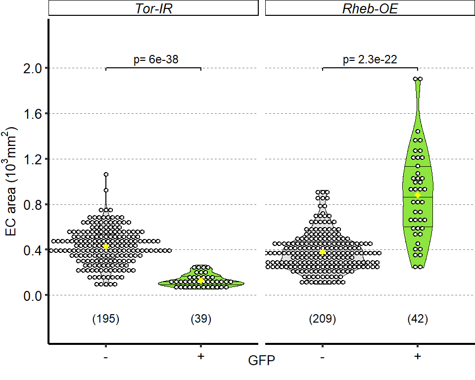
7.1.3 Figure 7E-F
Knockdown of TOR with MyoTS, an EC-specific driver, leads to the increased number of small ECs (F, right) compared to control (E, left); EC-specific GFP is indeed visible in small cells.Complete graphical annotation can be found in manuscript figures
img = readImage("F:/Dropbox/Github/Bonfini_eLife_2021/data/7E.jpg")
gob_imageFig7E = rasterGrob(img)
grid.draw(gob_imageFig7E)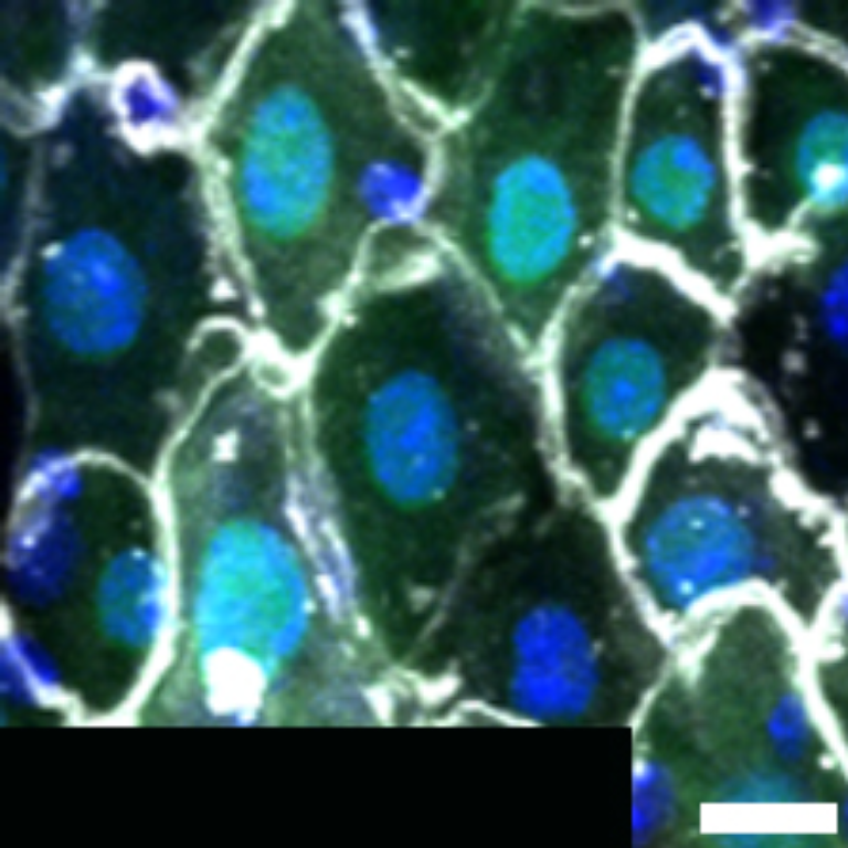
img = readImage("F:/Dropbox/Github/Bonfini_eLife_2021/data/7F.jpg")
gob_imageFig7F = rasterGrob(img)
grid.draw(gob_imageFig7F)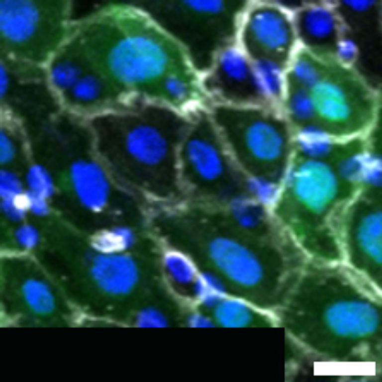
7.1.4 Figure 7G
Quantification of EC area. Statistic annotation on panel present in manuscript’s figure.
tab_area_Tor_IR =
d[["7G"]]%>%
mutate_at(vars(!starts_with("Area")),as.factor)%>%
dplyr::rename(Day_of_treatment=Day,
Female_Line=Female.Line,
Male_Line=Male.Line)%>%
as.data.frame()%>%
mutate(Diet=fct_relevel(Diet,c("HS", "HStoHY")),
Male_Line=fct_relevel(Male_Line,c("Control","Tor-IR")))
Sample_size=
tab_area_Tor_IR%>%
group_by(Diet,Male_Line)%>%
summarise(Sample_size=n())
###Stats Tor
# D7
mod.gen = fitme(log(Area) ~ Diet * Male_Line + (1 | Repeat ) ,data = tab_area_Tor_IR)
shapiro.test(residuals(mod.gen))
Shapiro-Wilk normality test
data: residuals(mod.gen)
W = 0.99748, p-value = 0.0005718bptest(log(Area) ~ Diet * Male_Line + (1 / Repeat ) ,data = tab_area_Tor_IR)
studentized Breusch-Pagan test
data: log(Area) ~ Diet * Male_Line + (1/Repeat)
BP = 37.175, df = 3, p-value = 4.225e-08mod.gen1 = fitme(log(Area) ~ Diet + Male_Line + (1 | Repeat ),data = tab_area_Tor_IR)
test = anova(mod.gen, mod.gen1)
Chi2_LRT_growth = 2*(mod.gen$APHLs[["p_v"]]-mod.gen1$APHLs[["p_v"]])
tab_stat = data.frame(Variable = as.character("Control vs Tor-IR"),
Rep = nlevels(tab_area_Tor_IR$Repeat),
chi2_LR = round(as.numeric(test$basicLRT$chi2_LR), digits = 2),
intercept = format(mod.gen$fixef[1],digits=3),
estimate = format(mod.gen$fixef[4],digits=3),
df = as.numeric(test$basicLRT$df),
Pvalue = as.numeric(format(pchisq(Chi2_LRT_growth,df=1,lower.tail = F),digits=2)))
tab_stat$sig = ifelse(tab_stat$Pvalue < 0.05 & tab_stat$Pvalue > 0.01, "*",
ifelse(tab_stat$Pvalue < 0.01 & tab_stat$Pvalue > 0.001, "**",
ifelse(tab_stat$Pvalue < 0.001, "***", "")))
tab_stat%>%
kable(col.names = c("Response to diet", "Replicates", "Chi2","Intercept","Estimate","df" ,"p-value","Signif."),row.names = FALSE) %>% add_header_above(c("log(Cell area) ~ Diet + Genotype + Diet : Genotype + (1 | Repeat)" = 8))%>%
kable_styling(bootstrap_options = c("striped", "hover", "condensed"), full_width = F)| Response to diet | Replicates | Chi2 | Intercept | Estimate | df | p-value | Signif. |
|---|---|---|---|---|---|---|---|
| Control vs Tor-IR | 3 | 178.09 | 4.61 | -0.491 | 1 | 0 | *** |
tab_stat_7E=tab_stat
tab_stat_7E$Male_Line=factor("Tor-IR", labels = c(expression(italic("Tor-IR"))))
tab_stat_7E$Diet=c("HStoHY")
tab_stat_7E$yposition = c(0.7)
tab_stat_7E$xposition = c(1.5)
### Plot
tab_area_Tor_IR$Female_Line = factor(tab_area_Tor_IR$Female_Line, labels = c(expression(italic(paste("My",o^{TS},">",sep="")))))
tab_area_Tor_IR$Male_Line = factor(tab_area_Tor_IR$Male_Line, labels = c(expression(italic("Control"),italic("Tor-IR"))))
Sample_size$Male_Line = factor(Sample_size$Male_Line, labels = c(expression(italic("Control"),italic("Tor-IR"))))
Plot_Fig7G=
ggplot(tab_area_Tor_IR, aes(x = Diet, y = Area/1000))+
geom_violin(aes(fill = C.G), draw_quantiles = c(0.25, 0.5, 0.75), colour = "black", size = 0.2,adjust = 5) +
geom_dotplot( colour = "black", fill = "white", binaxis = "y", stackdir = "center", binwidth = 0.008) +
geom_text(data = Sample_size, mapping = aes(x = Diet, y = -0.1, label = paste("(",Sample_size,")",sep="")),size=3)+
facet_grid(.~Male_Line,labeller=label_parsed )+
scale_fill_manual(values=c("#FFB4B4", "#CCCCFF"))+
scale_x_discrete("",
limits=c("HS","HStoHY"),
labels=c("HS","HS to HY"))+
scale_y_continuous(expression(paste("EC area (10"^3, "mm"^2,")",sep="")),
limits=c(-0.12,1),
breaks=seq(0,0.8,by=0.2))+
stat_summary(fun = mean, geom = "point", size = 3, shape = 18, colour = "black", aes(group = Repeat)) +
stat_summary(fun = mean, geom = "point", size = 2, shape = 18, aes(group = Repeat, colour = Repeat)) +
stat_summary(fun = mean, colour = "black", geom = "line", aes(group = Repeat)) +
scale_color_manual(values = palette_mean) +
theme(panel.grid.major.y = element_line(colour = grey(0.45), linetype = "dashed", size = 0.2),
panel.background = element_blank(),
axis.title.x = element_text(size=Smallfont,colour="black"),
axis.title.y = element_text(size=Smallfont,colour="black"),
axis.line.x = element_line(colour="black",size=0.75),
axis.line.y = element_line(colour="black",size=0.75),
axis.ticks.x = element_line(size = 0.75),
axis.ticks.y = element_line(size = 0.75),
axis.text.x = element_text(size=Smallfont,colour="black",angle=30,hjust=1),
axis.text.y = element_text(size=Smallfont,colour="black"),
plot.margin = unit(Margin, "cm"),
legend.direction = "vertical",
legend.box = "horizontal",
legend.position = "none",
legend.key.height = unit(0.4, "cm"),
legend.key.width= unit(0.6, "cm"),
legend.title = element_text(face="italic",size=Smallfont),
legend.key = element_rect(colour = 'white', fill = "white", linetype='dashed'),
legend.text = element_text(size=SuperSmallfont),
legend.background = element_rect(fill=NA),
strip.text = element_text(size =Smallfont, colour = "black",face="italic", margin = margin(t = 2, r = 0, b = 2, l = 0)),
strip.background = element_rect(fill=NA, colour="black"),
strip.placement="outside")
Plot_Fig7G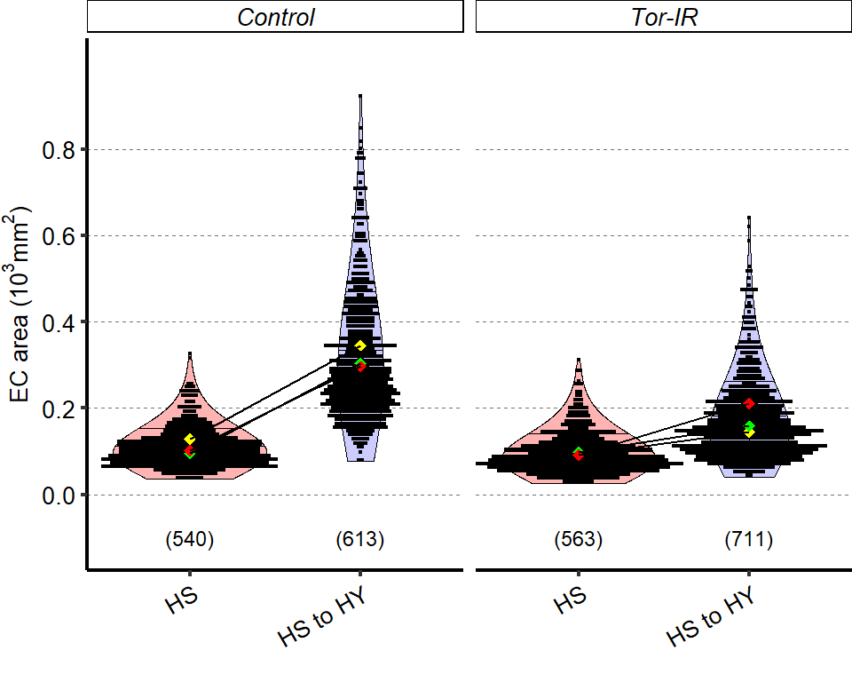
7.1.5 Figure 7H
Blocking TOR pathway components in ECs (MyoTS) inhibits diet induced midgut growth. Control showed in chart is representative of multiple experiments. Statistical analyses were performed only on appropriate repeat/experiment and comparing interaction between diet and fly line.
tab_length_Tor =
d[["7H"]]%>%
mutate_at(vars(!starts_with("Total")),as.factor)%>%
mutate(Total_Length_mm=Total.L/1000)%>%
dplyr::rename(Day_of_treatment=Day,
Female_Line=Female.Line,
Male_Line=Male.Line)%>%
as.data.frame()%>%
mutate(Male_Line=fct_relevel(Male_Line, "Control", "Tor-IR","dMyc-IR","S6k-IR", "SREBP-IR", "raptor-IR"))
Sample_size=
tab_length_Tor%>%
group_by(Diet,Male_Line)%>%
summarise(Sample_size=n())
###Stats
list_genotype= c("Tor-IR","dMyc-IR","S6k-IR", "SREBP-IR", "raptor-IR")
tab_stat_Tor=NULL
for (i in list_genotype){
list_control=
subset(tab_length_Tor,Male_Line%in%c(i)) %>%
mutate(PhaseRep=factor(PhaseRep))%>%
summarise(levels(PhaseRep))
list_control = as.list(list_control$`levels(PhaseRep)`)
tmp= subset(tab_length_Tor, Male_Line%in%c(i, "Control") & PhaseRep%in%list_control)%>%
mutate(Male_Line=factor(Male_Line),
PhaseRep=factor(PhaseRep))
mod.gen = fitme(log10(Total_Length_mm) ~ Diet * Male_Line + (1 | PhaseRep),data = tmp)
shapiro.test(residuals(mod.gen))
bptest(log10(Total_Length_mm) ~ Diet + Male_Line + (1 / PhaseRep),data = tmp)
mod.gen1 = fitme(log10(Total_Length_mm) ~ Diet + Male_Line + (1 | PhaseRep),data = tmp)
test = anova(mod.gen, mod.gen1)
test
Chi2_LRT_growth = 2*(mod.gen$APHLs[["p_v"]]-mod.gen1$APHLs[["p_v"]])
tab_stat = data.frame(Male_Line = as.character(i),
Rep = nlevels(tmp$PhaseRep),
chi2_LR = round(as.numeric(test$basicLRT$chi2_LR), digits = 2),
intercept = format(mod.gen$fixef[1],digits=3),
estimate = format(mod.gen$fixef[4],digits=3),
df = as.numeric(test$basicLRT$df),
Pvalue = as.numeric(format(pchisq(Chi2_LRT_growth,df=1,lower.tail = F),digits=2)))
tab_stat_Tor = rbind(tab_stat_Tor,tab_stat)
}
tab_stat_Tor$padj=p.adjust(tab_stat_Tor$Pvalue,method = "BH")
tab_stat_Tor$sig= ifelse(tab_stat_Tor$padj < 0.05 & tab_stat_Tor$padj > 0.01, "*",
ifelse(tab_stat_Tor$padj < 0.01 & tab_stat_Tor$padj > 0.001, "**",
ifelse(tab_stat_Tor$padj < 0.001, "***", "ns")))
tab_stat_Tor%>%
kable(col.names = c("Response to diet", "Replicates", "Chi2","Intercept","Estimate","df" ,"p-value","p-value adjusted","Signif."),row.names = FALSE) %>% add_header_above(c("log10(Total_Length_mm) ~ Diet + Genotype + Diet : Genotype + (1 | Repeat)" = 9))%>%
kable_styling(bootstrap_options = c("striped", "hover", "condensed"), full_width = F)| Response to diet | Replicates | Chi2 | Intercept | Estimate | df | p-value | p-value adjusted | Signif. |
|---|---|---|---|---|---|---|---|---|
| Tor-IR | 4 | 36.00 | 0.592 | -0.115 | 1 | 0.0000 | 0.0000000 | *** |
| dMyc-IR | 5 | 8.20 | 0.579 | -0.0462 | 1 | 0.0042 | 0.0088333 | ** |
| S6k-IR | 3 | 7.77 | 0.57 | -0.0478 | 1 | 0.0053 | 0.0088333 | ** |
| SREBP-IR | 3 | 5.93 | 0.58 | -0.0434 | 1 | 0.0150 | 0.0187500 |
|
| raptor-IR | 3 | 2.77 | 0.595 | -0.0303 | 1 | 0.0960 | 0.0960000 | ns |
tab_stat_Tor=
tab_stat_Tor%>%
as.data.frame()%>%
mutate(Male_Line=fct_relevel(Male_Line, "Tor-IR","dMyc-IR","S6k-IR", "SREBP-IR", "raptor-IR"))
### Plot
tab_length_Tor$Female_Line = factor(tab_length_Tor$Female_Line, labels = c(expression(italic(paste("My",o^{TS},">",sep="")))))
z = max(tab_length_Tor$Total_Length_mm, na.rm = TRUE)
Plot_Fig7H=
ggplot(tab_length_Tor, aes(x = Diet, y = Total_Length_mm))+
geom_violin(aes(fill = Diet), draw_quantiles = c(0.25, 0.5, 0.75), colour = "black", size = 0.2,adjust = 0.8) +
geom_dotplot( colour = "black", fill = "white", binaxis = "y", stackdir = "center", binwidth = z/80) +
geom_text(data = Sample_size, mapping = aes(x = Diet, y = 2.4, label = paste("(",Sample_size,")",sep="")),size=3)+
geom_text(data = tab_stat_Tor, mapping = aes(x = 1.5, y = 8.3, label = paste("p=",format(Pvalue,digits=2))),size=3)+
facet_grid(.~Male_Line )+
scale_fill_manual(values=cbbHS_HStoHY)+
scale_x_discrete("",
limits=c("HS","HStoHY"),
labels=c("HS","HS to HY"))+
scale_y_continuous("Midgut length (mm)",
limits=c(2,8.3),
breaks=seq(2,8,by=1))+
stat_summary(fun = mean, geom = "point", size = 3, shape = 18, colour = "black", aes(group = PhaseRep)) +
stat_summary(fun = mean, geom = "point", size = 2, shape = 18, aes(group = PhaseRep, colour = PhaseRep)) +
stat_summary(fun = mean, colour = "black", geom = "line", aes(group = PhaseRep)) +
scale_color_manual(values = palette_mean) +
theme(panel.grid.major.y = element_line(colour = grey(0.45), linetype = "dashed", size = 0.2),
panel.background = element_blank(),
axis.title.x = element_text(size=Smallfont,colour="black"),
axis.title.y = element_text(size=Smallfont,colour="black"),
axis.line.x = element_line(colour="black",size=0.75),
axis.line.y = element_line(colour="black",size=0.75),
axis.ticks.x = element_line(size = 0.75),
axis.ticks.y = element_line(size = 0.75),
axis.text.x = element_text(size=Smallfont,colour="black",angle=30,hjust=1),
axis.text.y = element_text(size=Smallfont,colour="black"),
plot.margin = unit(Margin, "cm"),
legend.direction = "vertical",
legend.box = "horizontal",
legend.position = "none",
legend.key.height = unit(0.4, "cm"),
legend.key.width= unit(0.6, "cm"),
legend.title = element_text(face="italic",size=Smallfont),
legend.key = element_rect(colour = 'white', fill = "white", linetype='dashed'),
legend.text = element_text(size=SuperSmallfont),
legend.background = element_rect(fill=NA),
strip.text.x = element_text(size = xSmallfont, colour = "black", angle=0, face = "italic", margin = margin(t = 2, r = 0, b = 2, l = 0)),
strip.text.y = element_text(size = xSmallfont, colour = "black", angle=0, face = "italic", margin = margin(t = 2, r = 0, b = 2, l = 0)),
strip.background = element_rect(fill=NA, colour="black"),
strip.placement="outside")
Plot_Fig7H
7.1.6 Figure 7I-J
:::
Representative picture utilizing single cell clonal system suggests that blocking Atg2 (hsFlp; Act>STOP>Gal4, UAS-GFP >UAS-Atg2-IR, GFP+ cells) results in bigger ECs compared to control GFP- cells, quantified in J Complete graphical annotation can be found in manuscript figures
img = readImage("F:/Dropbox/Github/Bonfini_eLife_2021/data/7I.jpg")
gob_imageFig7I = rasterGrob(img)
grid.draw(gob_imageFig7I)
:::
tab_ECclone_quant1 =
d[["7J"]]%>%
mutate_at(vars(!starts_with("Area")),as.factor)%>%
dplyr::rename(Male_Line=Male.Line)%>%
as.data.frame()
Sample_size=
tab_ECclone_quant1%>%
group_by(GFP)%>%
summarise(Sample_size=n())%>%
as.data.frame()
###Stats
mod.gen = fitme(log(Area) ~ GFP,data = subset(tab_ECclone_quant1, Male_Line=="Atg2-IR"))
shapiro.test(residuals(mod.gen))
Shapiro-Wilk normality test
data: residuals(mod.gen)
W = 0.98076, p-value = 0.6105bptest(log(Area) ~ GFP ,data = subset(tab_ECclone_quant1, Male_Line=="Atg2-IR"))
studentized Breusch-Pagan test
data: log(Area) ~ GFP
BP = 0.43242, df = 1, p-value = 0.5108mod.gen1 = fitme(log(Area) ~ 1 ,data = subset(tab_ECclone_quant1, Male_Line=="Atg2-IR"))
test = anova(mod.gen, mod.gen1)
Chi2_LRT_growth = 2*(mod.gen$APHLs[["p_v"]]-mod.gen1$APHLs[["p_v"]])
tab_stat = data.frame(Variable = as.character(paste("GFP Negative vs Positive (Atg2-IR)")),
chi2_LR = round(as.numeric(test$basicLRT$chi2_LR), digits = 2),
intercept = format(mod.gen$fixef[1],digits=3),
estimate = format(mod.gen$fixef[2],digits=3),
df = as.numeric(test$basicLRT$df),
Pvalue = as.numeric(format(pchisq(Chi2_LRT_growth,df=1,lower.tail = F),digits=2)))
tab_stat$sig = ifelse(tab_stat$Pvalue < 0.05 & tab_stat$Pvalue > 0.01, "*",
ifelse(tab_stat$Pvalue < 0.01 & tab_stat$Pvalue > 0.001, "**",
ifelse(tab_stat$Pvalue < 0.001, "***", "")))
tab_stat$Male_Line = as.factor(c("Atg2-IR"))
tab_stat%>%
kable(col.names = c("Comparison", "Chi2", "Intercept","Estimate","df" ,"p-value","Signif.", "RNAi line"),row.names = FALSE) %>% add_header_above(c("log(Cell area) ~ GFP" = 8))%>%
kable_styling(bootstrap_options = c("striped", "hover", "condensed"), full_width = F)| Comparison | Chi2 | Intercept | Estimate | df | p-value | Signif. | RNAi line |
|---|---|---|---|---|---|---|---|
| GFP Negative vs Positive (Atg2-IR) | 21.89 | 5.18 | 0.845 | 1 | 2.9e-06 | *** | Atg2-IR |
### Plot
Plot_Fig7J=
ggplot(tab_ECclone_quant1, aes(x = GFP, y = Area/1000))+
geom_violin(aes(fill = GFP), draw_quantiles = c(0.25, 0.5, 0.75), colour = "black", size = 0.2,adjust = 0.8) +
geom_dotplot( colour = "black", fill = "white", binaxis = "y", stackdir = "center", binwidth = 0.03) +
geom_text(data = Sample_size, mapping = aes(x = GFP, y = -0.08, label = paste("(",Sample_size,")",sep="")),size=3)+
geom_signif(data = tab_stat,aes(xmin = 1, xmax = 2, annotations = formatC(paste("p=",Pvalue), digits = 2), y_position = 0.9), textsize = 3, vjust = -0.2, manual = TRUE, tip_length = c(0.01, 0.01))+
facet_grid(.~Male_Line)+
scale_fill_manual(limits=c("No","Yes"),
values=c("#e4e4e4","#8ee53f"))+
scale_x_discrete("GFP",
limits=c("No","Yes"),
labels=c("-","+"))+
scale_y_continuous(expression(paste("EC area (10"^3, "mm"^2,")",sep="")),
limits=c(-0.1,1),
breaks=seq(0,2,by=0.4))+
stat_summary(fun = mean, geom = "point", size = 2, shape = 18, colour = "yellow") +
theme(panel.grid.major.y = element_line(colour = grey(0.45), linetype = "dashed", size = 0.2),
panel.background = element_blank(),
axis.title.x = element_text(size=Smallfont,colour="black"),
axis.title.y = element_text(size=Smallfont,colour="black"),
axis.line.x = element_line(colour="black",size=0.75),
axis.line.y = element_line(colour="black",size=0.75),
axis.ticks.x = element_line(size = 0.75),
axis.ticks.y = element_line(size = 0.75),
axis.text.x = element_text(size=Smallfont,colour="black",hjust=1),
axis.text.y = element_text(size=Smallfont,colour="black"),
plot.margin = unit(Margin, "cm"),
legend.direction = "vertical",
legend.box = "horizontal",
legend.position = "none",
legend.key.height = unit(0.4, "cm"),
legend.key.width= unit(0.6, "cm"),
legend.title = element_text(face="italic",size=Smallfont),
legend.key = element_rect(colour = 'white', fill = "white", linetype='dashed'),
legend.text = element_text(size=SuperSmallfont),
legend.background = element_rect(fill=NA),
strip.text.x = element_text(size = Smallfont, colour = "black", face="italic", margin = margin(t = 1, r = 0, b = 1, l = 0)),
strip.text.y = element_text(size = Smallfont, colour = "black", face="italic", margin = margin(t = 1, r = 0, b = 1, l = 0)),
strip.background = element_rect(fill=NA, colour="black"),
strip.placement="outside")
Plot_Fig7J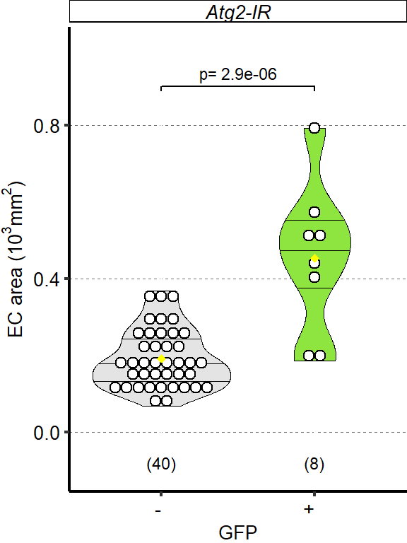
7.1.7 Figure 7K
Blocking autophagy reduces midgut resizing upon shrinkage (HY to HS for 7 days). Blocking Atg8a expression with RNAi in ECs (MyoTS> UAS-Atg8a-IR) results in less length shrinkage compared to control midguts.
tab_length_Atg8a =
d[["7K"]]%>%
mutate_at(vars(!starts_with("Total")),as.factor)%>%
mutate(Total_Length_mm=Total.L/1000)%>%
dplyr::rename(Day_of_treatment=Day,
Female_Line=Female.Line,
Male_Line=Male.Line)%>%
as.data.frame()%>%
mutate(Male_Line=fct_relevel(Male_Line,"Control","Atg8a-IR"))
Sample_size=
tab_length_Atg8a%>%
group_by(Diet,Male_Line)%>%
summarise(Sample_size=n())%>%
as.data.frame()%>%
mutate(Male_Line=fct_relevel(Male_Line,"Control","Atg8a-IR"))
###Stats
mod.gen = fitme(log10(Total_Length_mm) ~ Diet * Male_Line + (1 | PhaseRep),data = tab_length_Atg8a)
shapiro.test(residuals(mod.gen))
Shapiro-Wilk normality test
data: residuals(mod.gen)
W = 0.99618, p-value = 0.9774bptest(log10(Total_Length_mm) ~ Diet + Male_Line + (1 / PhaseRep),data = tab_length_Atg8a)
studentized Breusch-Pagan test
data: log10(Total_Length_mm) ~ Diet + Male_Line + (1/PhaseRep)
BP = 0.46985, df = 2, p-value = 0.7906mod.gen1 = fitme(log10(Total_Length_mm) ~ Diet + Male_Line + (1 | PhaseRep),data = tab_length_Atg8a)
test = anova(mod.gen, mod.gen1)
Chi2_LRT_growth = 2*(mod.gen$APHLs[["p_v"]]-mod.gen1$APHLs[["p_v"]])
tab_stat = data.frame(Comparison = as.character(paste("Interaction control vs interaction Atg8a-IR")),
Male_Line = as.character("Atg8a-IR"),
Rep = nlevels(tab_length_Atg8a$PhaseRep),
chi2_LR = round(as.numeric(test$basicLRT$chi2_LR), digits = 2),
intercept = format(mod.gen$fixef[1],digits=3),
estimate = format(mod.gen$fixef[4],digits=3),
df = as.numeric(test$basicLRT$df),
Pvalue = as.numeric(format(pchisq(Chi2_LRT_growth,df=1,lower.tail = F),digits=2)))%>%
mutate(Male_Line=fct_relevel(Male_Line,"Atg8a-IR"))
tab_stat$sig = ifelse(tab_stat$Pvalue < 0.05 & tab_stat$Pvalue > 0.01, "*",
ifelse(tab_stat$Pvalue < 0.01 & tab_stat$Pvalue > 0.001, "**",
ifelse(tab_stat$Pvalue < 0.001, "***", "")))
tab_stat%>%
kable(col.names = c("Comparison","Variable", "Replicates", "Chi2","Intercept","Estimate","df" ,"p-value","Signif."),row.names = FALSE) %>% add_header_above(c("log10(Total_Length_mm) ~ Diet + Genotype + Diet : Genotype + (1 | Repeat)" = 9))%>%
kable_styling(bootstrap_options = c("striped", "hover", "condensed"), full_width = F)| Comparison | Variable | Replicates | Chi2 | Intercept | Estimate | df | p-value | Signif. |
|---|---|---|---|---|---|---|---|---|
| Interaction control vs interaction Atg8a-IR | Atg8a-IR | 4 | 22.8 | 0.742 | 0.0782 | 1 | 1.8e-06 | *** |
tab_stat7K = tab_stat
### Plot
tab_length_Atg8a$Female_Line = factor(tab_length_Atg8a$Female_Line, labels = c(expression(italic(paste("My",o^{TS},">",sep="")))))
z = max(tab_length_Atg8a$Total_Length_mm, na.rm = TRUE)
Plot_Fig7K=
ggplot(tab_length_Atg8a, aes(x = Diet, y = Total_Length_mm))+
geom_violin(aes(fill = Diet), draw_quantiles = c(0.25, 0.5, 0.75), colour = "black", size = 0.2,adjust = 0.8) +
geom_dotplot( colour = "black", fill = "white", binaxis = "y", stackdir = "center", binwidth = z/60) +
geom_text(data = Sample_size, mapping = aes(x = Diet, y = 2.3, label = paste("(",Sample_size,")",sep="")),size=3)+
facet_grid(.~Male_Line)+
scale_fill_manual(values=cbbHY_HYtoHS)+
scale_x_discrete("",
limits=c("HY","HYtoHS"),
labels=c("HY","HY to HS"))+
scale_y_continuous("Midgut length (mm)",
limits=c(2,7.5),
breaks=seq(2,7,by=1))+
stat_summary(fun = mean, geom = "point", size = 2, shape = 18, aes(group = Repeat, colour = Repeat)) +
stat_summary(fun = mean, colour = "black", geom = "line", aes(group = Repeat)) +
scale_color_manual(values = palette_mean) +
theme(panel.grid.major.y = element_line(colour = grey(0.45), linetype = "dashed", size = 0.2),
panel.background = element_blank(),
axis.title.x = element_text(size=Smallfont,colour="black"),
axis.title.y = element_text(size=Smallfont,colour="black"),
axis.line.x = element_line(colour="black",size=0.75),
axis.line.y = element_line(colour="black",size=0.75),
axis.ticks.x = element_line(size = 0.75),
axis.ticks.y = element_line(size = 0.75),
axis.text.x = element_text(size=Smallfont,colour="black",angle=30,hjust=1),
axis.text.y = element_text(size=Smallfont,colour="black"),
plot.margin = unit(Margin, "cm"),
legend.direction = "vertical",
legend.box = "horizontal",
legend.position = "none",
legend.key.height = unit(0.4, "cm"),
legend.key.width= unit(0.6, "cm"),
legend.title = element_text(face="italic",size=Smallfont),
legend.key = element_rect(colour = 'white', fill = "white", linetype='dashed'),
legend.text = element_text(size=SuperSmallfont),
legend.background = element_rect(fill=NA),
strip.text.x = element_text(size = Smallfont, colour = "black", face="italic", margin = margin(t = 1, r = 0, b = 1, l = 0)),
strip.text.y = element_text(size = Smallfont, colour = "black", face="italic", margin = margin(t = 1, r = 0, b = 1, l = 0)),
strip.background = element_rect(fill=NA, colour="black"),
strip.placement="outside")
Plot_Fig7K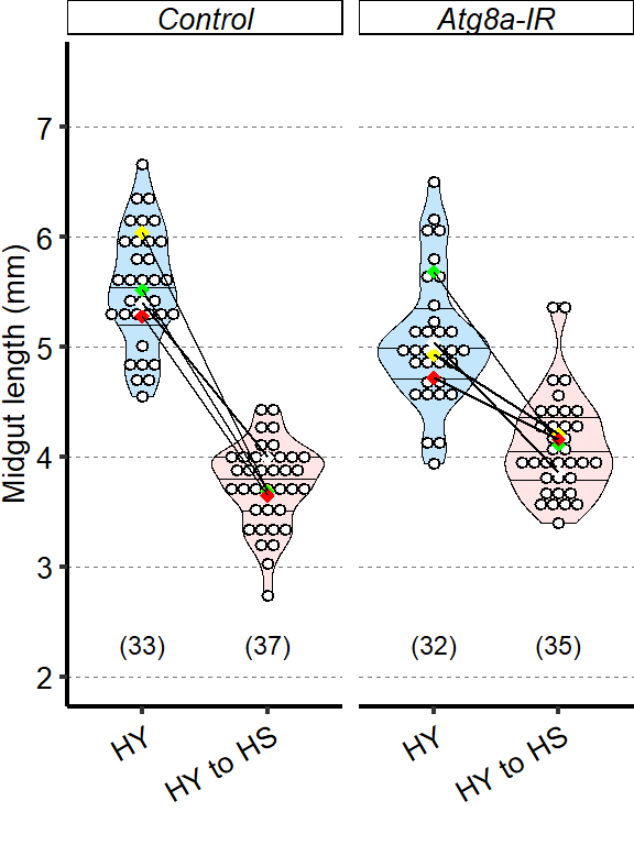
7.1.8 Figure 7L
Blocking Atg2 expression with RNAi in ECs (MyoTS> UAS-Atg2-IR) results in less width shrinkage compared to control midguts. Complete statistical annotation in manuscript’s figure.
tab_length_Atg2 =
d[["7L"]]%>%
mutate_at(vars(!starts_with("Total")),as.factor)%>%
mutate(Total_Width_mm=Total.W/1000)%>%
dplyr::rename(Day_of_treatment=Day,
Female_Line=Female.Line,
Male_Line=Male.Line)%>%
as.data.frame()%>%
mutate(Male_Line=fct_relevel(Male_Line,"Control","Atg2-IR"))
Sample_size=
tab_length_Atg2%>%
group_by(Diet,Male_Line)%>%
summarise(Sample_size=n())%>%
as.data.frame()%>%
mutate(Male_Line=fct_relevel(Male_Line,"Control","Atg2-IR"))
###Stats
mod.gen = fitme(log10(Total_Width_mm) ~ Diet * Male_Line + (1 | PhaseRep),data = tab_length_Atg2)
shapiro.test(residuals(mod.gen))
Shapiro-Wilk normality test
data: residuals(mod.gen)
W = 0.98933, p-value = 0.3713bptest(log10(Total_Width_mm) ~ Diet + Male_Line + (1 / PhaseRep),data = tab_length_Atg2)
studentized Breusch-Pagan test
data: log10(Total_Width_mm) ~ Diet + Male_Line + (1/PhaseRep)
BP = 0.49881, df = 2, p-value = 0.7793mod.gen1 = fitme(log10(Total_Width_mm) ~ Diet + Male_Line + (1 | PhaseRep),data = tab_length_Atg2)
test = anova(mod.gen, mod.gen1)
Chi2_LRT_growth = 2*(mod.gen$APHLs[["p_v"]]-mod.gen1$APHLs[["p_v"]])
tab_stat = data.frame(Comparison = as.character(paste("Interaction control vs interaction Atg2-IR")),Male_Line = as.character("Atg2-IR"),
Rep = nlevels(tab_length_Atg2$PhaseRep),
chi2_LR = round(as.numeric(test$basicLRT$chi2_LR), digits = 2),
intercept = format(mod.gen$fixef[1],digits=3),
estimate = format(mod.gen$fixef[4],digits=3),
df = as.numeric(test$basicLRT$df),
Pvalue = as.numeric(format(pchisq(Chi2_LRT_growth,df=1,lower.tail = F),digits=2)))%>%
mutate(Male_Line=fct_relevel(Male_Line,"Atg2-IR"))
tab_stat$sig = ifelse(tab_stat$Pvalue < 0.05 & tab_stat$Pvalue > 0.01, "*",
ifelse(tab_stat$Pvalue < 0.01 & tab_stat$Pvalue > 0.001, "**",
ifelse(tab_stat$Pvalue < 0.001, "***", "")))
tab_stat%>%
kable(col.names = c("Comparison", "Variable", "Replicates", "Chi2","Intercept","Estimate","df" ,"p-value","Signif."),row.names = FALSE) %>% add_header_above(c("log10(Total_width_mm) ~ Diet + Genotype + Diet : Genotype + (1 | Repeat)" = 9))%>%
kable_styling(bootstrap_options = c("striped", "hover", "condensed"), full_width = F)| Comparison | Variable | Replicates | Chi2 | Intercept | Estimate | df | p-value | Signif. |
|---|---|---|---|---|---|---|---|---|
| Interaction control vs interaction Atg2-IR | Atg2-IR | 4 | 10.74 | -0.267 | 0.0524 | 1 | 0.001 |
tab_stat7L = tab_stat
### Plot
tab_length_Atg2$Female_Line = factor(tab_length_Atg2$Female_Line, labels = c(expression(italic(paste("My",o^{TS},">",sep="")))))
z = max(tab_length_Atg2$Total_Width_mm, na.rm = TRUE)
Plot_Fig7L=
ggplot(tab_length_Atg2, aes(x = Diet, y = Total_Width_mm))+
geom_violin(aes(fill = Diet), draw_quantiles = c(0.25, 0.5, 0.75), colour = "black", size = 0.2,adjust = 0.8) +
geom_dotplot( colour = "black", fill = "white", binaxis = "y", stackdir = "center", binwidth = z/60) +
geom_text(data = Sample_size, mapping = aes(x = Diet, y = 0.24, label = paste("(",Sample_size,")",sep="")),size=3)+
# geom_text(data = tab_stat, mapping = aes(x = 1.5, y =0.88, label = paste("p=",Pvalue)),size=3)+
facet_grid(.~Male_Line)+
scale_fill_manual(values=cbbHY_HYtoHS)+
scale_x_discrete("",
limits=c("HY","HYtoHS"),
labels=c("HY","HY to HS"))+
scale_y_continuous("Midgut width (mm)",
limits=c(0.2,0.9),
breaks=seq(0.2,1,by=0.1))+
stat_summary(fun = mean, geom = "point", size = 2, shape = 18, aes(group = Repeat, colour = Repeat)) +
stat_summary(fun = mean, colour = "black", geom = "line", aes(group = Repeat)) +
scale_color_manual(values = palette_mean) +
theme(panel.grid.major.y = element_line(colour = grey(0.45), linetype = "dashed", size = 0.2),
panel.background = element_blank(),
axis.title.x = element_text(size=Smallfont,colour="black"),
axis.title.y = element_text(size=Smallfont,colour="black"),
axis.line.x = element_line(colour="black",size=0.75),
axis.line.y = element_line(colour="black",size=0.75),
axis.ticks.x = element_line(size = 0.75),
axis.ticks.y = element_line(size = 0.75),
axis.text.x = element_text(size=Smallfont,colour="black",angle=30,hjust=1),
axis.text.y = element_text(size=Smallfont,colour="black"),
plot.margin = unit(Margin, "cm"),
legend.direction = "vertical",
legend.box = "horizontal",
legend.position = "none",
legend.key.height = unit(0.4, "cm"),
legend.key.width= unit(0.6, "cm"),
legend.title = element_text(face="italic",size=Smallfont),
legend.key = element_rect(colour = 'white', fill = "white", linetype='dashed'),
legend.text = element_text(size=SuperSmallfont),
legend.background = element_rect(fill=NA),
strip.text.x = element_text(size = Smallfont, colour = "black", face="italic", margin = margin(t = 1, r = 0, b = 1, l = 0)),
strip.text.y = element_text(size = Smallfont, colour = "black", face="italic", margin = margin(t = 1, r = 0, b = 1, l = 0)),
strip.background = element_rect(fill=NA, colour="black"),
strip.placement="outside")
Plot_Fig7L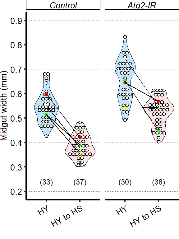
##Export Figure 7
7.2 Figure 7 - supplementary 1
7.2.1 Figure 7S1A
The midgut plastically resizes through changes in EC cell size. Quantification of EC area shows that, in addition to total length, the midgut is also able to plastically resize (Figure 4A) its own ECs. ECs scored are derived from midguts measured for length in figure 4A. Letters above violin plots represent grouping by statistical differences (Post hoc Tukey on GLMM).
tab_area_plasticity =
d[["7 - S1A"]]%>%
mutate_if(is.character,as.factor)%>%
mutate_if(is.integer,as.factor)
Sample_size=
tab_area_plasticity%>%
group_by(Diet)%>%
summarise(Sample_size=n())
###Stats
mod.gen = fitme(log10(Area) ~ Diet + (1 | Repeat), data = tab_area_plasticity)
shapiro.test(residuals(mod.gen))
Shapiro-Wilk normality test
data: residuals(mod.gen)
W = 0.99946, p-value = 0.6205bptest(log10(Area) ~ Diet + (1 / Repeat), data = tab_area_plasticity)
studentized Breusch-Pagan test
data: log10(Area) ~ Diet + (1/Repeat)
BP = 66.112, df = 3, p-value = 2.9e-14mod.gen1 = fitme(log10(Area) ~ 1 + (1 | Repeat), data = tab_area_plasticity)
test = anova(mod.gen, mod.gen1)
Chi2_LRT_growth = 2*(mod.gen$APHLs[["p_v"]]-mod.gen1$APHLs[["p_v"]])
tab_stat = data.frame(Variable = as.character(paste("Anova between diets")),
Rep = nlevels(tab_area_plasticity$Repeat),
chi2_LR = round(as.numeric(test$basicLRT$chi2_LR), digits = 2),
intercept = format(mod.gen$fixef[1],digits=2),
estimate = format(format(mod.gen$fixef[2],digits=3),digits=2),
df = as.numeric(test$basicLRT$df),
Pvalue = as.numeric(format(pchisq(Chi2_LRT_growth,df=1,lower.tail = F),digits=2,scientific=T)))
tab_stat$sig = ifelse(tab_stat$Pvalue < 0.05 & tab_stat$Pvalue > 0.01, "*",
ifelse(tab_stat$Pvalue < 0.01 & tab_stat$Pvalue > 0.001, "**",
ifelse(tab_stat$Pvalue < 0.001, "***", "")))
tab_stat%>%
kable(col.names = c("Variable", "Replicates", "Chi2","Intercept","Estimate","df" ,"p-value","Signif."),row.names = FALSE) %>% add_header_above(c("log10(Cell area) ~ Diet + (1 | Repeat)" = 8))%>%
kable_styling(bootstrap_options = c("striped", "hover", "condensed"), full_width = F)| Variable | Replicates | Chi2 | Intercept | Estimate | df | p-value | Signif. |
|---|---|---|---|---|---|---|---|
| Anova between diets | 3 | 1514.68 | 2.1 | 0.395 | 3 | 0 | *** |
mod.gen = lmer(log10(Area) ~ Diet + (1 | Repeat), data = tab_area_plasticity)
multcomp = glht(mod.gen, linfct=mcp(Diet="Tukey"))
tmp = cld(multcomp)
letter_position = aggregate(data=tab_area_plasticity,I(Area/1000) ~ Diet, max)
tab_letter = as.data.frame(tmp$mcletters$Letters)
tab_letter$Diet=rownames(tab_letter)
colnames(tab_letter)[1] = "Letter"
tab_letter = left_join(tab_letter,letter_position)
colnames(tab_letter)[3] = "Area"
### Plot
z = max(tab_area_plasticity$Area/1000, na.rm = TRUE)
Plot_Fig7S1A=
ggplot(tab_area_plasticity, aes(x = Diet, y = Area/1000))+
geom_violin(aes(fill = Diet), draw_quantiles = c(0.25, 0.5, 0.75), colour = "black", size = 0.2) +
geom_dotplot( colour = "black", fill = "white", binaxis = "y", stackdir = "center", binwidth = z/300) +
geom_text(data = Sample_size, mapping = aes(x = Diet, y = -0.01, label = paste("(",Sample_size,")",sep="")),size=3)+
geom_text(data = tab_stat, mapping = aes(x = 1, y =1.15, label = paste("p< ",format(.Machine$double.xmin,digits=2))),size=3)+
geom_text(data = tab_letter, mapping = aes(x = Diet, y = Area+0.05, label = Letter),size=3)+
scale_fill_manual(limits=c("Eclosion", "HY", "HYtoHS", "HYtoHStoHY"),
values= cbbPalette_4 )+
scale_x_discrete("",
limits=c("Eclosion", "HY", "HYtoHS", "HYtoHStoHY"),
labels=c("Eclosion", "HY", "HY to HS", "HY to HS to HY"))+
scale_y_continuous(expression(paste("EC area (10"^3, "mm"^2,")",sep="")),
limits=c(-0.01,1.22),
breaks=seq(0,1.2,by=0.1))+
stat_summary(fun = mean, geom = "point", size = 2, shape = 18, aes(group = Repeat, colour = Repeat)) +
scale_color_manual(values = palette_mean) +
theme(
panel.grid.major.y = element_line(colour = grey(0.45), linetype = "dashed", size = 0.2),
panel.background = element_blank(),
axis.title.x = element_text(size=Smallfont,colour="black"),
axis.title.y = element_text(size=Smallfont,colour="black"),
axis.line.x = element_line(colour="black",size=0.75),
axis.line.y = element_line(colour="black",size=0.75),
axis.ticks.x = element_line(size = 0.75),
axis.ticks.y = element_line(size = 0.75),
axis.text.x = element_text(size=Smallfont,colour="black",angle=15,hjust=1),
axis.text.y = element_text(size=Smallfont,colour="black"),
plot.margin = unit(Margin, "cm"),
legend.direction = "vertical",
legend.box = "horizontal",
legend.position = "none",
legend.key.height = unit(0.4, "cm"),
legend.key.width= unit(0.6, "cm"),
legend.title = element_text(face="italic",size=Smallfont),
legend.key = element_rect(colour = 'white', fill = "white", linetype='dashed'),
legend.text = element_text(size=SuperSmallfont),
legend.background = element_rect(fill=NA))
Plot_Fig7S1A
7.2.2 Figure 7S1B
Changes in EC area between HS and HY (ratio HY/HS of mean EC area) significantly correlate with changes in midgut size between HS and HY (ratio HY/HS of mean midgut length) across selected DGRP lines.
tab_corr_length_cell_DGRP_mean_area =
tab_corr_length_cell_DGRP%>%
group_by(ral,diet)%>%
summarise(mean_area=mean(ec.area,na.rm=T))%>%
spread(diet,mean_area)%>%
dplyr::rename(mean_area_HS=HS,
mean_area_HY=HY)%>%
mutate(Ratio_area = mean_area_HY/mean_area_HS)
tab_corr_length_cell_DGRP_mean_length =
tab_corr_length_cell_DGRP%>%
group_by(ral,diet)%>%
summarise(mean_length=mean(len,na.rm=T))%>%
spread(diet,mean_length)%>%
dplyr::rename(mean_length_HS=HS,
mean_length_HY=HY)%>%
mutate(Ratio_length = mean_length_HY/mean_length_HS)
tab_corr_length_cell_DGRP_mean= left_join(tab_corr_length_cell_DGRP_mean_length,tab_corr_length_cell_DGRP_mean_area)
tab_corr_length_cell_DGRP_mean=as.data.frame(tab_corr_length_cell_DGRP_mean)
levels(tab_corr_length_cell_DGRP_mean$ral) <- c("Ral 356", "Ral 362", "Ral 370", "Ral 502", "Ral 765", "Ral 853", "Ral 911" )
test =
with(tab_corr_length_cell_DGRP_mean,
cor.test(Ratio_area,Ratio_length,method="pearson"))
tab_stat = data.frame(Statistic = test$statistic,
cor = test$estimate,
Pvalue = test$p.value)
#levels(tab_corr_length_cell_DGRP_mean$ral) <- c("Ral 356", "Ral 362", "Ral 370", "Ral 502", "Ral 765", "Ral 853", "Ral 911" )
Plot_Fig7S1B =
ggplot(tab_corr_length_cell_DGRP_mean,aes(x=Ratio_area,y=Ratio_length,label=ral))+
geom_point()+
scale_x_continuous(expression(paste("Ratio HY/HS (mean EC area)")),
limits=c(0.8,2.6),
breaks=c(seq(0.8,2.8,by=0.2)))+
scale_y_continuous("Ratio HY/HS (mean midgut length)",
limits=c(0.8,2.6),
breaks=c(seq(0.8,2.8,by=0.2)))+
geom_text_repel(data=tab_corr_length_cell_DGRP_mean,size=3)+
geom_smooth(method="lm")+
geom_text(data = tab_stat, mapping = aes(x = 1.7, y = 1.7, label = paste("cor=", format(cor, digits=2), "p=",format(Pvalue,digits=2))),size=3)+
theme(panel.grid.major.y = element_line(colour = grey(0.45), linetype = "dashed", size = 0.2),
panel.background = element_blank(),
(panel.border = element_blank()),
axis.title.x = element_text(size=Smallfont,colour="black"),
axis.title.y = element_text(size=Smallfont,colour="black"),
axis.line.x = element_line(colour="black",size=0.75),
axis.line.y = element_line(colour="black",size=0.75),
axis.ticks.x = element_blank(),
axis.ticks.y = element_line(size = 0.75),
axis.text.x = element_text(size=Smallfont,colour="black"),
axis.text.y = element_text(size=Smallfont,colour="black"),
plot.margin = unit(Margin, "cm"),
legend.direction = "horizontal",
legend.box = "horizontal",
legend.position = c(0.25,0.98),
legend.key.height = unit(0.4, "cm"),
legend.key.width= unit(0.4, "cm"),
legend.title = element_blank(),
legend.key = element_rect(colour = 'white', fill = "white", linetype='dashed'),
legend.text = element_text(size=Smallfont),
legend.background = element_rect(fill=NA))+
guides(color=guide_legend(ncol=3))
Plot_Fig7S1B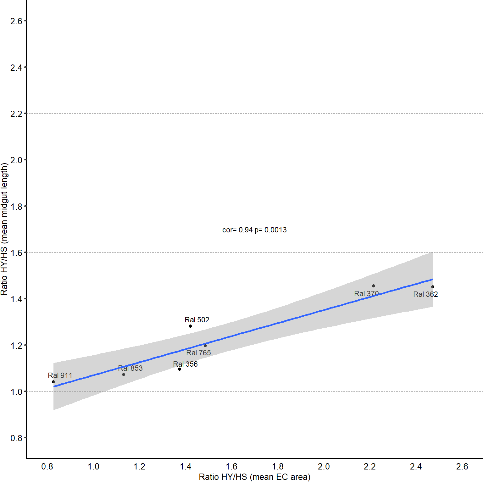
##Export Figure 7S1
7.3 Figure 7 - supplementary 2
7.3.1 Figure 7S2A-B
A reporter line for Foxo pathway activity, thor-lacZ, has increased intensity on HS (A, A’) compared to HY (B, B’). Quantification of mean pixel intensity of thor-lacZ stain (C). Complete graphical annotation can be found in manuscript figures
img = readImage("F:/Dropbox/Github/Bonfini_eLife_2021/data/7- S2A.jpg")
gob_imageFig7S2A = rasterGrob(img)
grid.draw(gob_imageFig7S2A)
img = readImage("F:/Dropbox/Github/Bonfini_eLife_2021/data/7- S2A1.jpg")
gob_imageFig7S2A1 = rasterGrob(img)
grid.draw(gob_imageFig7S2A1)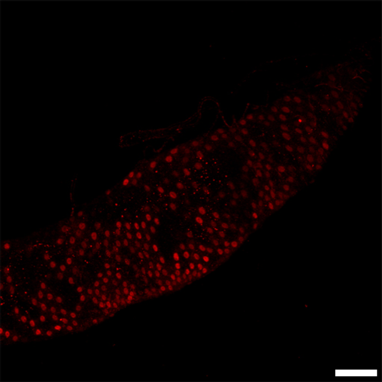
img = readImage("F:/Dropbox/Github/Bonfini_eLife_2021/data/7- S2B.jpg")
gob_imageFig7S2B = rasterGrob(img)
grid.draw(gob_imageFig7S2B)
img = readImage("F:/Dropbox/Github/Bonfini_eLife_2021/data/7- S2B1.jpg")
gob_imageFig7S2B1 = rasterGrob(img)
grid.draw(gob_imageFig7S2B1)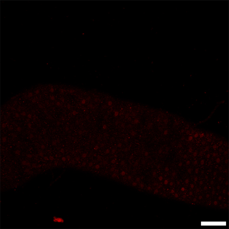
7.3.2 Figure 7S2C
Quantification thor-lacZ
tab_ThorlacZ_rev =
d[["7 - S2C"]]%>%
mutate_if(is.character,as.factor)%>%
mutate_if(is.integer,as.factor)%>%
dplyr::rename(ThorlacZ_int=Mean)
Sample_size=
tab_ThorlacZ_rev%>%
group_by(Diet)%>%
summarise(Sample_size=n())
###Stats
mod.gen = fitme(log(ThorlacZ_int) ~ Diet + (1 | Repeat),data = tab_ThorlacZ_rev)
shapiro.test(residuals(mod.gen))
Shapiro-Wilk normality test
data: residuals(mod.gen)
W = 0.96119, p-value = 0.1441bptest(log(ThorlacZ_int) ~ Diet + (1 / Repeat),data = tab_ThorlacZ_rev)
studentized Breusch-Pagan test
data: log(ThorlacZ_int) ~ Diet + (1/Repeat)
BP = 10.584, df = 1, p-value = 0.001141mod.gen1 = fitme(log(ThorlacZ_int) ~ 1 + (1 | Repeat),data = tab_ThorlacZ_rev)
test = anova(mod.gen, mod.gen1)
Chi2_LRT = 2*(mod.gen$APHLs[["p_v"]]-mod.gen1$APHLs[["p_v"]])
tab_stat = data.frame(Variable = as.character(paste("HS vs HY")),
Rep = nlevels(tab_ThorlacZ_rev$Repeat),
chi2_LR = round(as.numeric(test$basicLRT$chi2_LR), digits = 2),
intercept = format(mod.gen$fixef[1],digits=3),
estimate = format(mod.gen$fixef[2],digits=3),
df = as.numeric(test$basicLRT$df),
Pvalue = as.numeric(format(pchisq(Chi2_LRT,df=1,lower.tail = F),digits=2)))
tab_stat$sig = ifelse(tab_stat$Pvalue < 0.05 & tab_stat$Pvalue > 0.01, "*",
ifelse(tab_stat$Pvalue < 0.01 & tab_stat$Pvalue > 0.001, "**",
ifelse(tab_stat$Pvalue < 0.001, "***", "")))
tab_stat%>%
kable(col.names = c("Comparison", "Replicates", "Chi2","Intercept","Estimate","df" ,"p-value","Signif."),row.names = FALSE) %>% add_header_above(c("log(Thor-lacZ intensity) ~ Diet + (1 | Repeat)" = 8))%>%
kable_styling(bootstrap_options = c("striped", "hover", "condensed"), full_width = F)| Comparison | Replicates | Chi2 | Intercept | Estimate | df | p-value | Signif. |
|---|---|---|---|---|---|---|---|
| HS vs HY | 3 | 40.09 | 2.96 | -1.07 | 1 | 0 | *** |
### Plot
Plot_Fig7S2C=
ggplot(tab_ThorlacZ_rev, aes(x = Diet, y = ThorlacZ_int))+
geom_violin(aes(fill = Diet), draw_quantiles = c(0.25, 0.5, 0.75), colour = "black", size = 0.2,adjust = 0.8) +
geom_dotplot( colour = "black", fill = "white", binaxis = "y", stackdir = "center", binwidth = 0.8) +
geom_text(data = Sample_size, mapping = aes(x = Diet, y = -3, label = paste("(",Sample_size,")",sep="")),size=3)+
geom_signif(annotation = formatC(paste("p=",tab_stat$Pvalue), digits = 2), textsize = 3, y_position = 32, xmin = 1, xmax = 2, tip_length = c(0.02, 0.02), vjust = -0.2)+
scale_fill_manual(limits=c("HS","HY"),
values=c("#FFB4B4","#C3E6FC"))+
scale_x_discrete("",
limits=c("HS","HY"),
labels=c("HS","HY"))+
scale_y_continuous(bquote(atop("Mean pixel intensity" ,~ italic (Thor-lacZ) ~ "(a.u.)")),
limits=c(-5,35),
breaks=seq(0,30,by=10))+
stat_summary(fun = mean, geom = "point", size = 3, shape = 18, colour = "black", aes(group = Repeat)) +
stat_summary(fun = mean, geom = "point", size = 2, shape = 18, aes(group = Repeat, colour = Repeat)) +
scale_color_manual(values = palette_mean) +
theme(panel.grid.major.y = element_line(colour = grey(0.45), linetype = "dashed", size = 0.2),
panel.background = element_blank(),
axis.title.x = element_text(size=Smallfont,colour="black"),
axis.title.y = element_text(size=Smallfont,colour="black"),
axis.line.x = element_line(colour="black",size=0.75),
axis.line.y = element_line(colour="black",size=0.75),
axis.ticks.x = element_line(size = 0.75),
axis.ticks.y = element_line(size = 0.75),
axis.text.x = element_text(size=Smallfont,colour="black"),
axis.text.y = element_text(size=Smallfont,colour="black"),
plot.margin = unit(Margin, "cm"),
legend.direction = "vertical",
legend.box = "horizontal",
legend.position = "none",
legend.key.height = unit(0.4, "cm"),
legend.key.width= unit(0.6, "cm"),
legend.title = element_text(face="italic",size=Smallfont),
legend.key = element_rect(colour = 'white', fill = "white", linetype='dashed'),
legend.text = element_text(size=SuperSmallfont),
legend.background = element_rect(fill=NA),
strip.text = element_text(size =Smallfont-2, colour = "black",face="italic", margin = margin(t = 2, r = 0, b = 2, l = 0)),
strip.background = element_rect(fill=NA, colour="black"),
strip.placement="outside")
Plot_Fig7S2C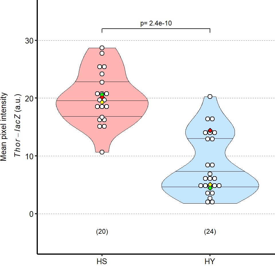
7.3.3 Figure 7S2D
Blocking TOR in ECs (5966GS> UAS-Tor-IR) inhibits diet induced midgut growth. For control we used flies of the same genotype but not exposed to RU486. Statistical analyses were performed by comparing interaction between diet and fly line.
tab_5966TOR_rev =
d[["7 - S2D"]]%>%
mutate_at(vars(!starts_with("Total")),as.factor)%>%
mutate(Total_Length_mm=Total.L/1000)%>%
dplyr::rename(Day_of_treatment=Day,
Female_Line=Female.Line,
Male_Line=Male.Line)%>%
mutate(Treatment=fct_relevel(Treatment,"Ethanol","RU486"))
Sample_size=
tab_5966TOR_rev%>%
group_by(Diet,Treatment)%>%
summarise(Sample_size=n())
###Stats
mod.gen = fitme(log(Total_Length_mm) ~ Diet * Treatment + (1 | Repeat),data =tab_5966TOR_rev)
shapiro.test(residuals(mod.gen))
Shapiro-Wilk normality test
data: residuals(mod.gen)
W = 0.98854, p-value = 0.4511bptest(log(Total_Length_mm) ~ Diet + Treatment + (1 / Repeat),data =tab_5966TOR_rev)
studentized Breusch-Pagan test
data: log(Total_Length_mm) ~ Diet + Treatment + (1/Repeat)
BP = 4.1422, df = 2, p-value = 0.126mod.gen1 = fitme(log(Total_Length_mm) ~ Diet + Treatment + (1 | Repeat),data =tab_5966TOR_rev)
test = anova(mod.gen, mod.gen1)
Chi2_LRT_growth = 2*(mod.gen$APHLs[["p_v"]]-mod.gen1$APHLs[["p_v"]])
tab_stat = data.frame(Variable = as.character(paste("Interaction ethanol vs interaction RU486")),
Rep = nlevels(tab_5966TOR_rev$Repeat),
chi2_LR = round(as.numeric(test$basicLRT$chi2_LR), digits = 2),
intercept = format(mod.gen$fixef[1],digits=3),
estimate = format(mod.gen$fixef[2],digits=3),
df = as.numeric(test$basicLRT$df),
Pvalue = as.numeric(format(pchisq(Chi2_LRT_growth,df=1,lower.tail = F),digits=2)))
tab_stat$sig = ifelse(tab_stat$Pvalue < 0.05 & tab_stat$Pvalue > 0.01, "*",
ifelse(tab_stat$Pvalue < 0.01 & tab_stat$Pvalue > 0.001, "**",
ifelse(tab_stat$Pvalue < 0.001, "***", "")))
tab_stat%>%
kable(col.names = c("Comparison", "Replicates", "Chi2","Intercept","Estimate","df" ,"p-value","Signif."),row.names = FALSE) %>% add_header_above(c("log(Total_Length_mm) ~ Diet + Treatment + Diet : Treatment + (1 | Repeat)" = 8))%>%
kable_styling(bootstrap_options = c("striped", "hover", "condensed"), full_width = F)| Comparison | Replicates | Chi2 | Intercept | Estimate | df | p-value | Signif. |
|---|---|---|---|---|---|---|---|
| Interaction ethanol vs interaction RU486 | 3 | 31.29 | 1.35 | 0.319 | 1 | 0 | *** |
tab_stat_rev_RU486=tab_stat
tab_stat_rev_RU486$Treatment="RU486"
tab_stat_rev_RU486$Treatment=as.factor(tab_stat_rev_RU486$Treatment)
### Plot
Plot_Fig7S2D =
ggplot(tab_5966TOR_rev, aes(x = Diet, y = Total_Length_mm))+
geom_violin(aes(fill = Diet), draw_quantiles = c(0.25, 0.5, 0.75), colour = "black", size = 0.2,adjust = 0.8) +
geom_dotplot( colour = "black", fill = "white", binaxis = "y", stackdir = "center", binwidth = 0.11) +
geom_text(data = Sample_size, mapping = aes(x = Diet, y = 2.2, label = paste("(",Sample_size,")",sep="")),size=3)+
stat_summary(fun = mean, geom = "point", size = 2, shape = 18,aes(group=Repeat, colour = Repeat)) +
stat_summary(fun = mean, geom = "point", size = 3, shape = 18, colour = "black", aes(group = Repeat)) +
stat_summary(fun = mean, geom = "point", size = 2, shape = 18, aes(group = Repeat, colour = Repeat)) +
stat_summary(fun = mean, colour = "black", geom = "line", aes(group = Repeat)) +
scale_color_manual(values = palette_mean) +
facet_grid(.~ Treatment)+
scale_fill_manual(values=cbbHS_HStoHY)+
scale_x_discrete("",
limits=c("HS D0","HStoHY D7"),
labels=c("HS","HS to HY"))+
scale_y_continuous("Midgut length (mm)",
limits=c(2,7),
breaks=seq(2,7,by=1))+
theme(panel.grid.major.y = element_line(colour = grey(0.45), linetype = "dashed", size = 0.2),
panel.background = element_blank(),
axis.title.x = element_text(size=Smallfont,colour="black"),
axis.title.y = element_text(size=Smallfont,colour="black"),
axis.line.x = element_line(colour="black",size=0.75),
axis.line.y = element_line(colour="black",size=0.75),
axis.ticks.x = element_line(size = 0.75),
axis.ticks.y = element_line(size = 0.75),
axis.text.x = element_text(size=Smallfont,colour="black",angle=30,hjust=1),
axis.text.y = element_text(size=Smallfont,colour="black"),
plot.margin = unit(Margin, "cm"),
legend.direction = "vertical",
legend.box = "horizontal",
legend.position = "none",
legend.key.height = unit(0.4, "cm"),
legend.key.width= unit(0.6, "cm"),
legend.title = element_text(face="italic",size=Smallfont),
legend.key = element_rect(colour = 'white', fill = "white", linetype='dashed'),
legend.text = element_text(size=SuperSmallfont),
legend.background = element_rect(fill=NA),
strip.text.x = element_text(size = Smallfont, colour = "black", face = "italic", margin = margin(t = 2, r = 0, b = 2, l = 0)),
strip.text.y = element_text(size = Smallfont, colour = "black", face = "italic", margin = margin(t = 2, r = 0, b = 2, l = 0)),
strip.background = element_rect(fill=NA, colour="black"),
strip.placement="outside")
Plot_Fig7S2D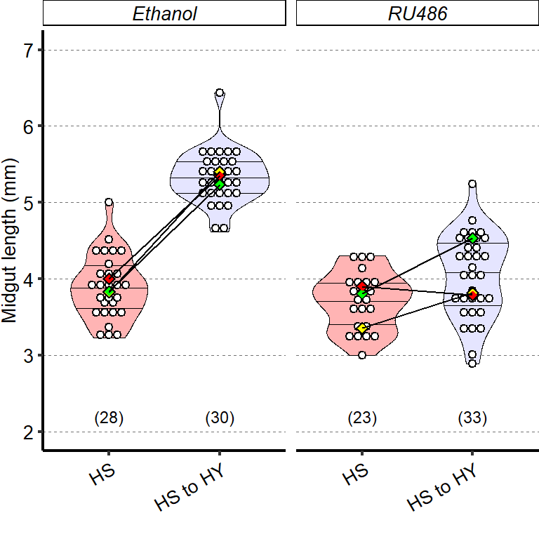
7.3.4 Figure 7S2E
Blocking autophagy in ECs reduces midgut resizing upon shrinkage (HY to HS for 7 days) using 5966GS> UAS-Atg8a-IR. For control we used flies of the same genotype but not exposed to RU486. Statistical analyses were performed by comparing interaction between diet and fly line. Complete statistical annotation can be found in manuscript’s figure.
tab_5966atg8a_rev =
d[["7 - S2E"]]%>%
mutate_at(vars(!starts_with("Total")),as.factor)%>%
mutate(Total_Length_mm=Total.L/1000)%>%
dplyr::rename(Day_of_treatment=Day,
Female_Line=Female.Line,
Male_Line=Male.Line)%>%
mutate(Treatment=fct_relevel(Treatment,"Ethanol","RU486"))
Sample_size=
tab_5966atg8a_rev%>%
group_by(Male_Line,Diet,Treatment)%>%
summarise(Sample_size=n())
###Stats
mod.gen = fitme(log10(Total_Length_mm) ~ Diet * Treatment + (1 | Repeat),data = tab_5966atg8a_rev)
shapiro.test(residuals(mod.gen))
Shapiro-Wilk normality test
data: residuals(mod.gen)
W = 0.9768, p-value = 0.06449bptest(log10(Total_Length_mm) ~ Diet * Treatment + (1 / Repeat),data = tab_5966atg8a_rev)
studentized Breusch-Pagan test
data: log10(Total_Length_mm) ~ Diet * Treatment + (1/Repeat)
BP = 5.6695, df = 3, p-value = 0.1288mod.gen1 = fitme(log10(Total_Length_mm) ~ Diet + Treatment + (1 | Repeat),data = tab_5966atg8a_rev)
test = anova(mod.gen, mod.gen1)
test chi2_LR df p_value
p_v 5.112911 1 0.02374845Chi2_LRT_growth = 2*(mod.gen$APHLs[["p_v"]]-mod.gen1$APHLs[["p_v"]])
tab_stat = data.frame(Comparison = as.character(paste("Interaction ethanol vs interaction RU486")),
Male_Line = as.character(paste("Atg8a-IR")),
Rep = nlevels(tab_5966atg8a_rev$Repeat),
chi2_LR = round(as.numeric(test$basicLRT$chi2_LR), digits = 2),
intercept = format(mod.gen$fixef[1],digits=3),
estimate = format(mod.gen$fixef[2],digits=3),
df = as.numeric(test$basicLRT$df),
Pvalue = as.numeric(format(pchisq(Chi2_LRT_growth,df=1,lower.tail = F),digits=1,scientific=F)))
tab_stat$sig = ifelse(tab_stat$Pvalue < 0.05 & tab_stat$Pvalue > 0.01, "*",
ifelse(tab_stat$Pvalue < 0.01 & tab_stat$Pvalue > 0.001, "**",
ifelse(tab_stat$Pvalue < 0.001, "***", "")))
tab_stat%>%
kable(col.names = c("Comparison","Variable", "Replicates", "Chi2", "Intercept","Estimate","df" ,"p-value","Signif."),row.names = FALSE) %>%
add_header_above(c("log(Total_Length_mm) ~ Diet + Treatment + Diet : Treatment + (1 | Repeat)" = 9))%>%
kable_styling(bootstrap_options = c("striped", "hover", "condensed"), full_width = F)| Comparison | Variable | Replicates | Chi2 | Intercept | Estimate | df | p-value | Signif. |
|---|---|---|---|---|---|---|---|---|
| Interaction ethanol vs interaction RU486 | Atg8a-IR | 3 | 5.11 | 0.767 | -0.118 | 1 | 0.02 |
|
tab_stat_5966atg8a_rev=tab_stat
tab_stat_5966atg8a_rev$Treatment="RU486"
tab_stat_5966atg8a_rev$Treatment=as.factor(tab_stat_rev_RU486$Treatment)
### Plot
Plot_Fig7S2E =
ggplot(tab_5966atg8a_rev, aes(x = Diet, y = Total_Length_mm))+
geom_violin(aes(fill = Diet), draw_quantiles = c(0.25, 0.5, 0.75), colour = "black", size = 0.2,adjust = 0.8) +
geom_dotplot( colour = "black", fill = "white", binaxis = "y", stackdir = "center", binwidth = 0.11) +
geom_text(data = Sample_size, mapping = aes(x = Diet, y = 2.2, label = paste("(",Sample_size,")",sep="")),size=3)+
stat_summary(fun = mean, geom = "point", size = 2, shape = 18,aes(group=Repeat, colour = Repeat)) +
stat_summary(fun = mean, geom = "point", size = 3, shape = 18, colour = "black", aes(group = Repeat)) +
stat_summary(fun = mean, geom = "point", size = 2, shape = 18, aes(group = Repeat, colour = Repeat)) +
stat_summary(fun = mean, colour = "black", geom = "line", aes(group = Repeat)) +
scale_color_manual(values = palette_mean) +
facet_grid(~ Treatment)+
scale_fill_manual(values=cbbHY_HYtoHS)+
scale_x_discrete("",
limits=c("HY","HYtoHS"),
labels=c("HY","HY to HS"))+
scale_y_continuous("Midgut length (mm)",
limits=c(2,8),
breaks=seq(2,8,by=1))+
theme(panel.grid.major.y = element_line(colour = grey(0.45), linetype = "dashed", size = 0.2),
panel.background = element_blank(),
axis.title.x = element_text(size=Smallfont,colour="black"),
axis.title.y = element_text(size=Smallfont,colour="black"),
axis.line.x = element_line(colour="black",size=0.75),
axis.line.y = element_line(colour="black",size=0.75),
axis.ticks.x = element_line(size = 0.75),
axis.ticks.y = element_line(size = 0.75),
axis.text.x = element_text(size=Smallfont,colour="black",angle=30,hjust=1),
axis.text.y = element_text(size=Smallfont,colour="black"),
plot.margin = unit(Margin, "cm"),
legend.direction = "vertical",
legend.box = "horizontal",
legend.position = "none",
legend.key.height = unit(0.4, "cm"),
legend.key.width= unit(0.6, "cm"),
legend.title = element_text(face="italic",size=Smallfont),
legend.key = element_rect(colour = 'white', fill = "white", linetype='dashed'),
legend.text = element_text(size=SuperSmallfont),
legend.background = element_rect(fill=NA),
strip.text.x = element_text(size = Smallfont, colour = "black", face = "italic", margin = margin(t = 2, r = 0, b = 2, l = 0)),
strip.text.y = element_text(size = Smallfont, colour = "black", face = "italic", margin = margin(t = 2, r = 0, b = 2, l = 0)),
strip.background = element_rect(fill=NA, colour="black"),
strip.placement="outside")
Plot_Fig7S2E
##Export Figure 7S2
7.4 Figure 7 - supplementary 3
7.4.1 Figure 7S3A
Scheme depicting the regulation of midgut size in response to dietary changes. EC size, together with the balance between cell gain and cell loss, determine midgut size. Diet can influence these three parameters, thus influencing midgut size. Yeast promotes midgut growth, and sugar antagonizes it. Sugar inhibits translation and uncouples ISC proliferation from expression of stress-derived pro-mitotic signals, thus resulting in smaller guts.
img = readImage("F:/Dropbox/Github/Bonfini_eLife_2021/data/7 - S3A.jpg")
gob_imageFig7S3A = rasterGrob(img)
grid.draw(gob_imageFig7S3A)
##Export Figure 7S3
sessionInfo()R version 4.1.0 (2021-05-18)
Platform: x86_64-w64-mingw32/x64 (64-bit)
Running under: Windows 10 x64 (build 19043)
Matrix products: default
locale:
[1] LC_COLLATE=French_France.1252 LC_CTYPE=French_France.1252
[3] LC_MONETARY=French_France.1252 LC_NUMERIC=C
[5] LC_TIME=French_France.1252
attached base packages:
[1] parallel stats4 grid stats graphics grDevices utils
[8] datasets methods base
other attached packages:
[1] ggsignif_0.6.2 plotfunctions_1.4
[3] kableExtra_1.3.4 knitr_1.33
[5] ggplotify_0.1.0 coxme_2.2-16
[7] bdsmatrix_1.3-4 DESeq2_1.32.0
[9] SummarizedExperiment_1.22.0 Biobase_2.52.0
[11] MatrixGenerics_1.4.3 matrixStats_0.60.1
[13] GenomicRanges_1.44.0 GenomeInfoDb_1.28.0
[15] IRanges_2.26.0 S4Vectors_0.30.0
[17] BiocGenerics_0.38.0 ggh4x_0.2.0
[19] forcats_0.5.1 metR_0.11.0
[21] ggrepel_0.9.1 multcomp_1.4-17
[23] TH.data_1.0-10 mvtnorm_1.1-2
[25] gridGraphics_0.5-1 RColorBrewer_1.1-2
[27] gplots_3.1.1 EBImage_4.34.0
[29] fields_12.5 viridis_0.6.1
[31] viridisLite_0.4.0 spam_2.7-0
[33] dotCall64_1.0-1 lme4_1.1-27.1
[35] Matrix_1.3-3 spaMM_3.8.0
[37] data.table_1.14.0 phia_0.2-1
[39] tidyr_1.1.3 scales_1.1.1
[41] stringr_1.4.0 dplyr_1.0.7
[43] xlsx_0.6.5 xlsxjars_0.6.1
[45] rJava_1.0-5 doBy_4.6.10
[47] psych_2.1.6 nparLD_2.1
[49] agricolae_1.3-5 gridExtra_2.3
[51] plotrix_3.8-1 survival_3.2-11
[53] ggplot2_3.3.5 lmtest_0.9-38
[55] zoo_1.8-9 car_3.0-10
[57] carData_3.0-4 MASS_7.3-54
[59] lattice_0.20-44 reshape2_1.4.4
[61] devtools_2.4.2 usethis_2.0.1
[63] workflowr_1.6.2
loaded via a namespace (and not attached):
[1] bit64_4.0.5 DelayedArray_0.18.0 KEGGREST_1.32.0
[4] RCurl_1.98-1.3 generics_0.1.0 callr_3.7.0
[7] RSQLite_2.2.7 combinat_0.0-8 proxy_0.4-26
[10] bit_4.0.4 webshot_0.5.2 xml2_1.3.2
[13] lubridate_1.7.10 httpuv_1.6.1 assertthat_0.2.1
[16] xfun_0.24 hms_1.1.0 jquerylib_0.1.4
[19] evaluate_0.14 promises_1.2.0.1 fansi_0.5.0
[22] caTools_1.18.2 readxl_1.3.1 DBI_1.1.1
[25] geneplotter_1.70.0 tmvnsim_1.0-2 htmlwidgets_1.5.3
[28] purrr_0.3.4 ellipsis_0.3.2 backports_1.2.1
[31] annotate_1.70.0 ROI_1.0-0 vctrs_0.3.8
[34] remotes_2.4.1 abind_1.4-5 cachem_1.0.5
[37] withr_2.4.2 checkmate_2.0.0 prettyunits_1.1.1
[40] mnormt_2.0.2 svglite_2.0.0 cluster_2.1.2
[43] crayon_1.4.1 genefilter_1.74.0 labeling_0.4.2
[46] pkgconfig_2.0.3 slam_0.1-48 nlme_3.1-152
[49] pkgload_1.2.2 rlang_0.4.11 questionr_0.7.4
[52] lifecycle_1.0.0 miniUI_0.1.1.1 sandwich_3.0-1
[55] registry_0.5-1 cellranger_1.1.0 rprojroot_2.0.2
[58] tiff_0.1-8 boot_1.3-28 whisker_0.4
[61] processx_3.5.2 png_0.1-7 bitops_1.0-7
[64] KernSmooth_2.23-20 Biostrings_2.60.1 blob_1.2.1
[67] jpeg_0.1-8.1 klaR_0.6-15 memoise_2.0.0
[70] magrittr_2.0.1 plyr_1.8.6 zlibbioc_1.38.0
[73] compiler_4.1.0 cli_3.0.1 XVector_0.32.0
[76] pbapply_1.4-3 ps_1.6.0 mgcv_1.8-35
[79] tidyselect_1.1.1 stringi_1.6.2 highr_0.9
[82] yaml_2.2.1 locfit_1.5-9.4 sass_0.4.0
[85] tools_4.1.0 rio_0.5.27 rstudioapi_0.13
[88] foreign_0.8-81 git2r_0.28.0 farver_2.1.0
[91] digest_0.6.27 shiny_1.6.0 Rcpp_1.0.7
[94] microbenchmark_1.4-7 broom_0.7.8 later_1.2.0
[97] httr_1.4.2 AnnotationDbi_1.54.1 Deriv_4.1.3
[100] colorspace_2.0-2 rvest_1.0.0 XML_3.99-0.6
[103] fs_1.5.0 splines_4.1.0 yulab.utils_0.0.2
[106] sessioninfo_1.1.1 systemfonts_1.0.2 xtable_1.8-4
[109] jsonlite_1.7.2 nloptr_1.2.2.2 AlgDesign_1.2.0
[112] testthat_3.1.0 R6_2.5.0 pillar_1.6.1
[115] htmltools_0.5.1.1 mime_0.11 glue_1.4.2
[118] fastmap_1.1.0 minqa_1.2.4 BiocParallel_1.26.2
[121] fftwtools_0.9-11 codetools_0.2-18 maps_3.3.0
[124] pkgbuild_1.2.0 utf8_1.2.1 bslib_0.2.5.1
[127] tibble_3.1.2 numDeriv_2016.8-1.1 curl_4.3.2
[130] gtools_3.9.2 zip_2.2.0 openxlsx_4.2.4
[133] rmarkdown_2.9 desc_1.4.0 curry_0.1.1
[136] munsell_0.5.0 GenomeInfoDbData_1.2.6 labelled_2.8.0
[139] haven_2.4.1 gtable_0.3.0